5 Sample size superpowers

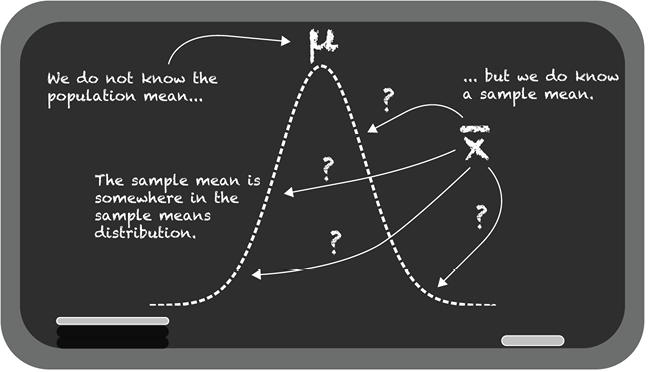
In practice, statistics usually begins with imperfect samples rather than complete populations, so the goal is to make the best possible estimate while being honest about uncertainty. This chapter shows how the central limit theorem supports that goal by describing how sample means form a bell-shaped distribution centered on the population mean, with spread that shrinks as sample size grows. That shrinking spread is the key to why larger samples produce more stable, predictable results and why confidence intervals are more precise when more data are available.

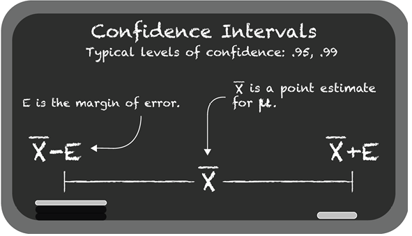
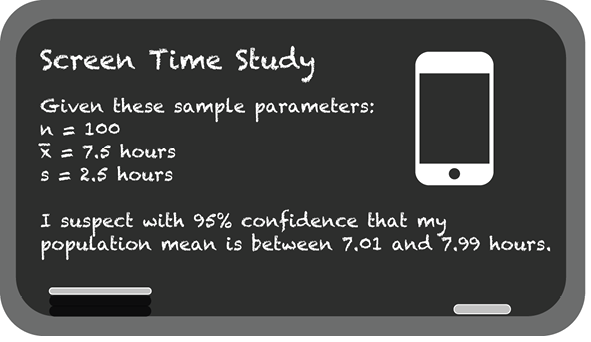
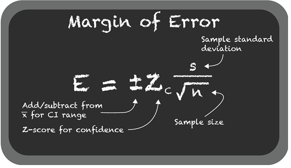
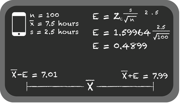
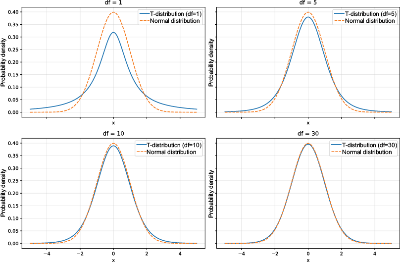
The chapter then turns this theory into a practical tool for estimating unknown population means. A point estimate gives a single best guess, but a confidence interval gives a range that is likely to contain the true value, built from the sample mean, a critical value, and the standard error. For large samples, the normal distribution is used to find the critical value; for smaller samples, the t-distribution is preferred because it accounts for extra uncertainty. The chapter emphasizes that a higher confidence level makes the interval wider, while a larger sample size makes it narrower.

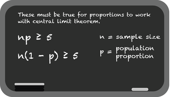
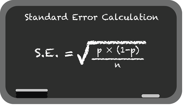
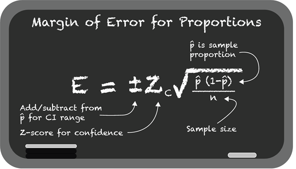
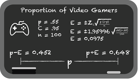
The same logic is extended to population proportions. When the outcome is categorical, such as yes/no behavior, the sample proportion can be modeled with the central limit theorem if the sample is large enough and the usual conditions are met. Confidence intervals for proportions follow the same general structure as those for means, but use the proportion-based standard error. Across all cases, the central message is that statistical inference is about describing uncertainty well, not pretending to know the truth with certainty.

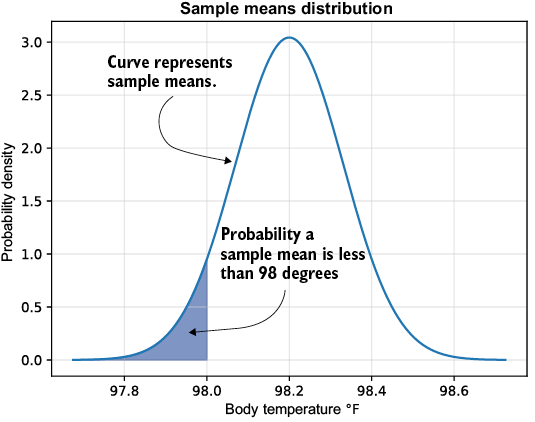
Plotting the sample means and visualizing the probability of a sample mean being less than 98 degrees

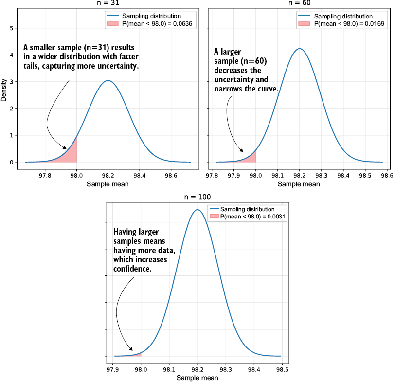
Increasing the sample size n narrows the bell curve and decreases uncertainty in the sample means.

What range of Z-values (on the horizontal axis) will give me a center, symmetrical area of .95?

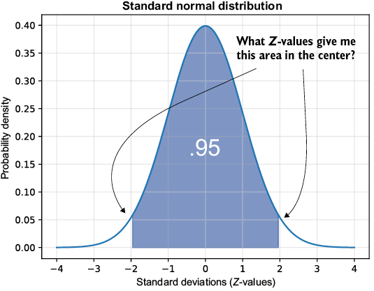
Breaking down the center .95 area in the bell curve and demonstrating the symmetry

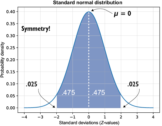
We need to look up the Z-value that captures the .025 area.

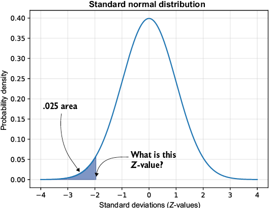
To find that right edge Z-value, we can add up .95 and .025 and look up that area, .975, in the PPF.

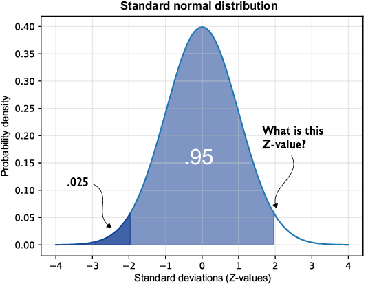
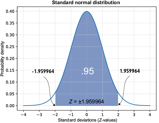
We have now captured our critical Z-value of ±1.959964.

The t-distribution with different degrees of freedom (DOF). Note that as the degrees of freedom approach 30, the distribution converges to a normal distribution.

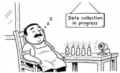
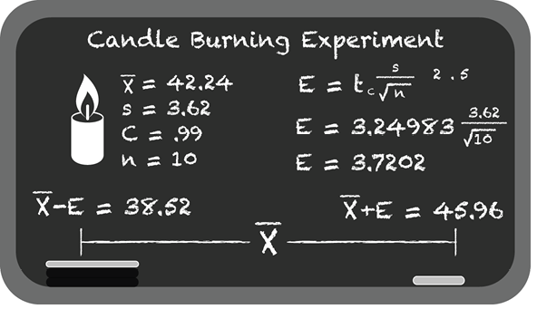
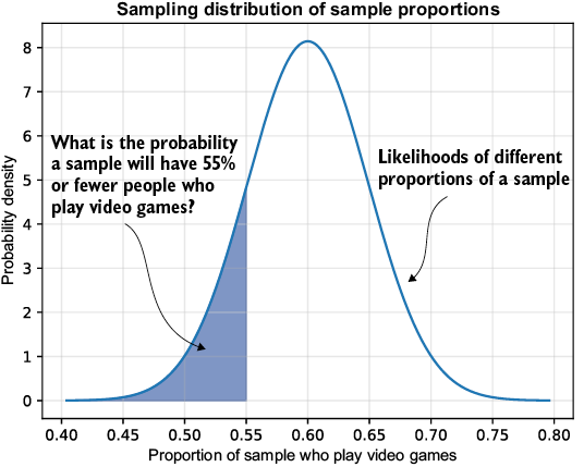
Modeling the sampling distribution of sample proportions, assigning different likelihoods to proportions of a sample

• The central limit theorem (CLT) allows us to tie a sample to a distribution of sample means or sample proportions, enabling tools such as confidence intervals (CIs) to estimate population parameters.
• Critical Z-values allow us to find a central, symmetrical area in a standard normal distribution, which can be utilized for CIs.
• CIs allow us to estimate a population’s mean or proportion from a sample using a range of values with a specified level of confidence, such as 95% or 99%.
• The t-distribution allows us to handle smaller samples when trying to estimate a population mean.

FAQ