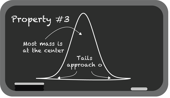
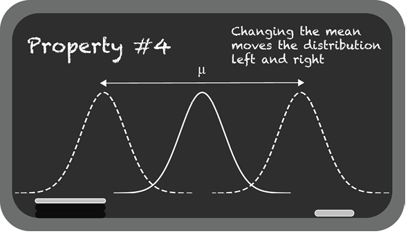
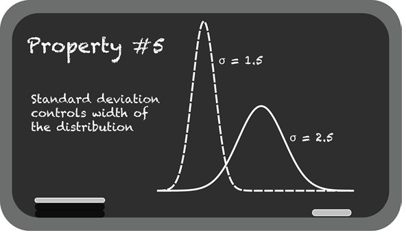
The chapter introduces the normal distribution as one of the most important ideas in statistics, with a symmetric bell shape governed by its mean and standard deviation. Through intuitive examples like human height and coffee preferences, it shows how the curve concentrates most values near the center and tapers into the tails, making it useful for describing real-world variation and for modeling data as a continuous probability distribution.
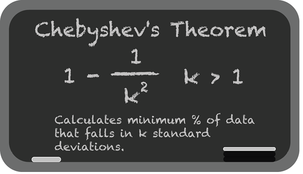
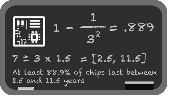
It then explains how to work with that curve mathematically and visually. The mean shifts the distribution left or right, the standard deviation controls its spread, and the total area under the curve remains 1. The chapter shows how probabilities are not tied to single exact values in a continuous distribution, but instead to intervals of area under the curve, and how cumulative distribution functions make those probability calculations practical. It also presents the empirical rule, which gives quick approximations for the proportions of data within one, two, and three standard deviations of the mean, and contrasts it with Chebyshev’s theorem, which provides a looser guarantee for nonnormal data.
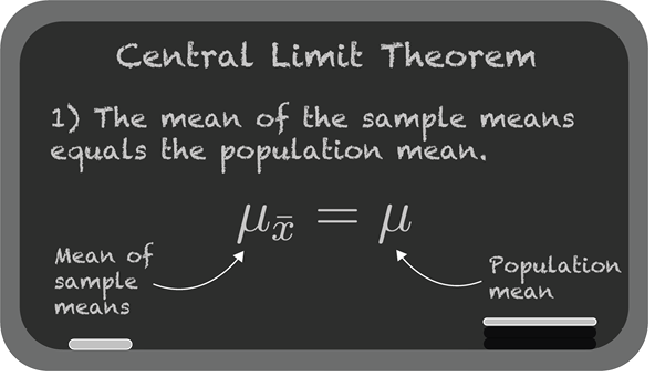
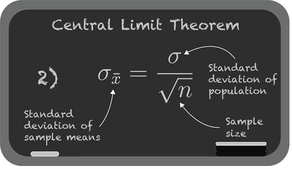
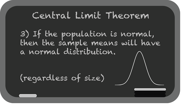
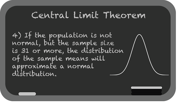
Finally, the chapter highlights the central limit theorem as a powerful bridge between samples and populations: repeated sample means tend to form a normal distribution even when the underlying data is skewed or irregular, especially for sufficiently large samples. This idea supports later statistical inference and is paired with standard normal distributions and Z-scores, which express values in standard-deviation units. The chapter closes by noting that some skewed data become approximately normal after a logarithmic transformation, leading to log-normal behavior in phenomena such as growth, income, and tornado width.
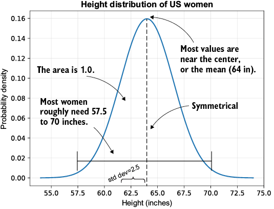
Normal distribution showing the height of US women
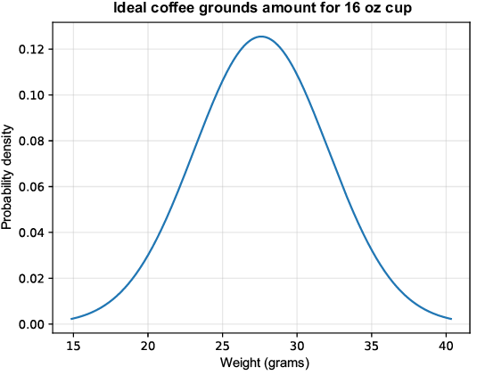
Surveying baristas on how many grams create a perfect 16 fl oz cup of coffee
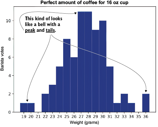
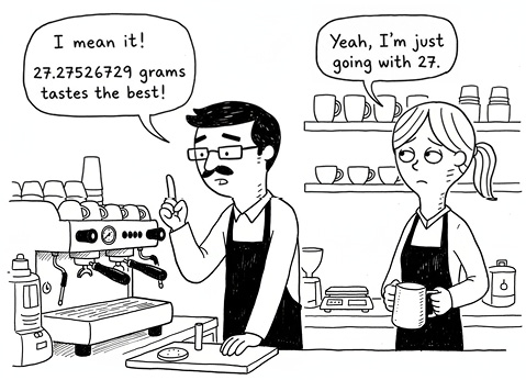
Plotting the normal distribution by scaling down the y-axis so the bell curve has an area of 1.0
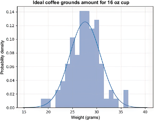
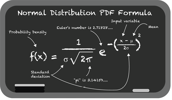
Plotting the normal distribution PDF using our from-scratch formula
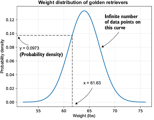
Looking up the probability density value for a golden retriever weight of 61.63 pounds
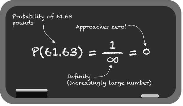
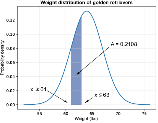
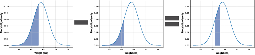
Looking up the probability/area for a golden retriever between 61 and 63 pounds
Getting the area up to 63 pounds
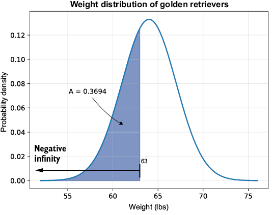
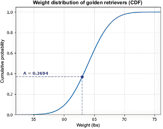
Getting the area up to 63 pounds, plotting the CDF
Subtracting areas using the CDF to get a middle range of area/probability
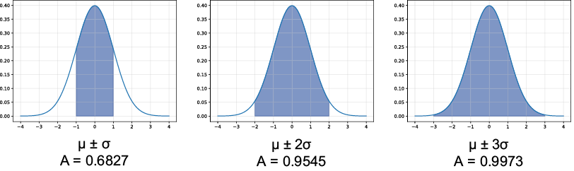
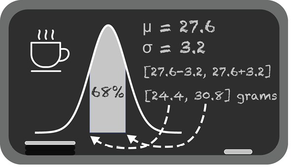
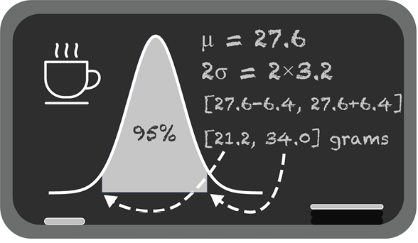
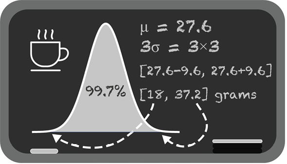
The empirical rule of the standard deviation

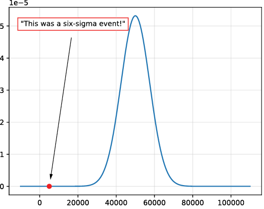
An investor blames an unlikely six-sigma event for a misfortune.

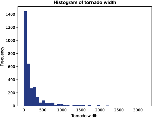
Tornado width is highly skewed to the right.
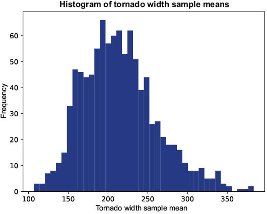
Tornado width sample means plotted as a histogram
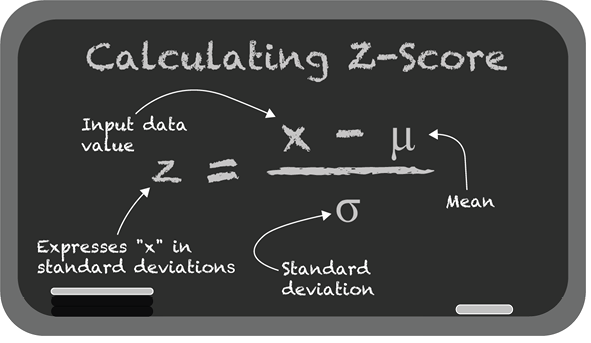
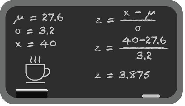
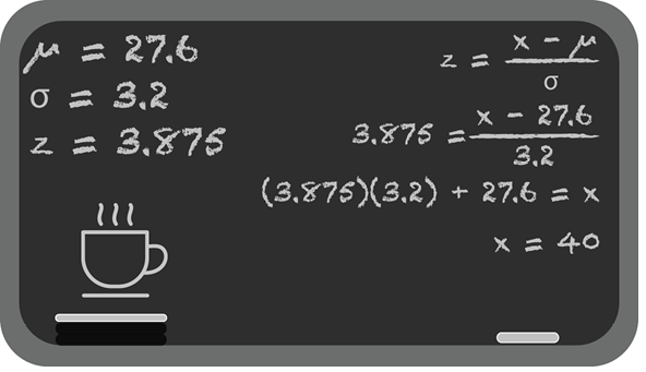
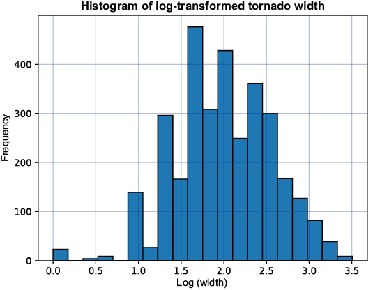
Treating the tornado width data with a logarithm gives it a normal distribution shape.
Summary
- The normal distribution is arguably the most important distribution, capturing many types of data that form a symmetrical bell curve determined by a mean and standard deviation.
- Like any probability distribution, the normal distribution calculates probability as areas over given ranges, which can be computed using cumulative distribution functions (CDFs).
- The normal distribution has several important properties, including the empirical rule for getting a sense of how much data falls within 1, 2, and 3 standard deviations of the mean.
- The central limit theorem (CLT) mathematically connects a sample to a population, allowing us to infer attributes of the population from sample means.
- The normal distribution appears even in nonnormal data, including the CLT and log-normal distributions.

 Grokking Statistics ebook for free
