9 Splitting data by asking questions: Decision trees

This chapter introduces decision trees as intuitive, interpretable models for both classification and regression. A decision tree predicts by asking a sequence of yes/no questions (decision nodes) and returning the label or value stored at a leaf. The structure consists of a root node, internal decision nodes, and leaf nodes, and it naturally mirrors human reasoning: partition the data by answering one question at a time. Trees can handle categorical features (by turning them into binary questions, e.g., via one-hot encoding) and continuous features (by selecting thresholds that split values), and the final prediction for a sample is the majority class (classification) or the average target (regression) at the reached leaf.

Training proceeds top-down with a greedy algorithm that picks, at each node, the split that best separates the data according to a chosen metric. For classification, the chapter compares accuracy, Gini impurity, and entropy (information gain), emphasizes weighted averages when branches differ in size, and shows how non-binary categories and numeric features translate into multiple candidate binary splits. To prevent overfitting, it introduces practical stopping criteria and hyperparameters such as maximum depth, minimum samples per split/leaf, and minimum impurity decrease, and demonstrates how to build and visualize trees with scikit-learn. For regression trees, the same top-down process is used but splits are chosen to minimize mean squared error, producing piecewise-constant predictions and axis-aligned boundaries in low dimensions.

Through worked examples—an app recommendation toy problem, a 2D geometric dataset, and a real university admissions dataset—the chapter highlights decision trees’ dual strengths: competitive predictive performance and clear interpretability (e.g., revealing which features and thresholds drive decisions). It shows how unrestricted trees can overfit and how tuning depth and sample-based constraints improves generalization. A compact regression example predicts app engagement by age with simple, readable segments. Finally, the chapter surveys impactful applications in healthcare and recommendation systems, and points ahead to ensemble methods (such as random forests and gradient-boosted trees) that combine many trees to further boost accuracy while retaining much of the interpretability and practical utility introduced here.

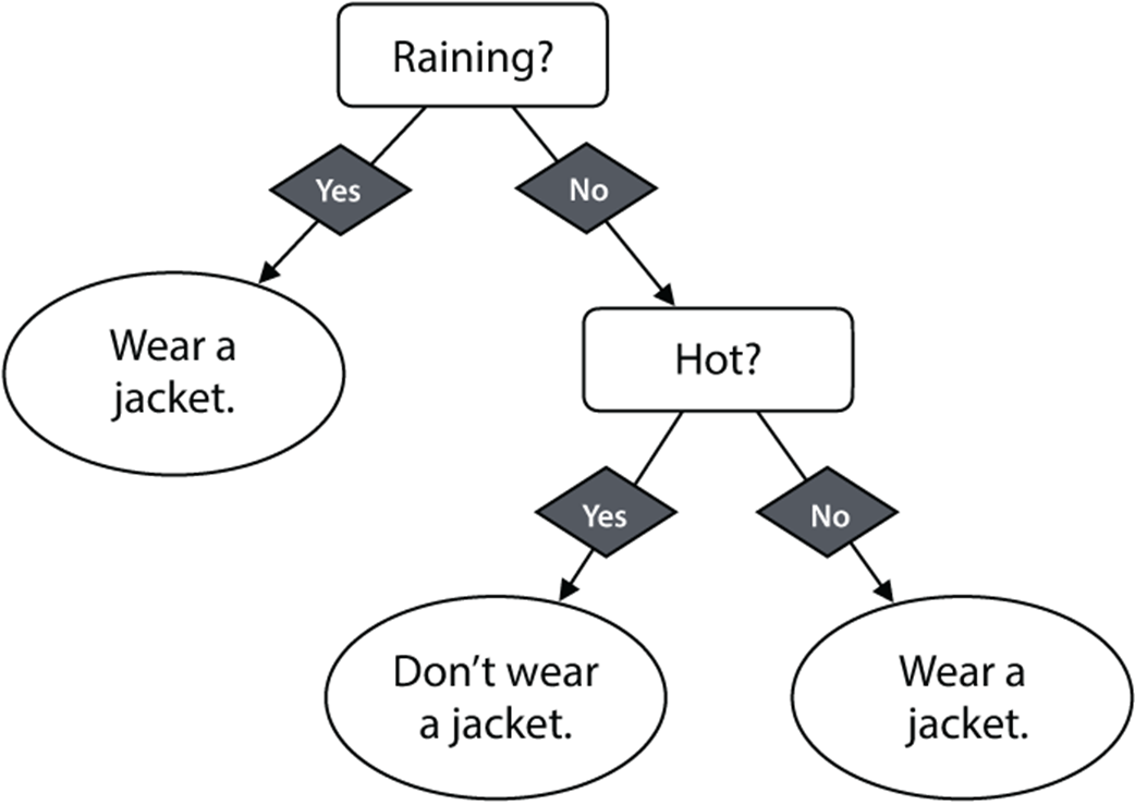
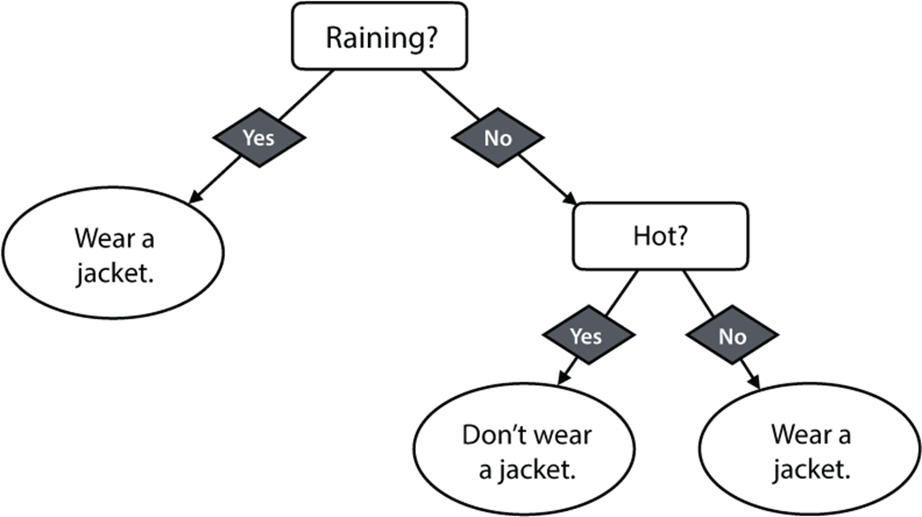
A decision tree used to decide whether we want to wear a jacket or not on a given day. We make the decision by traversing the tree down and taking the branch corresponding to each correct answer.

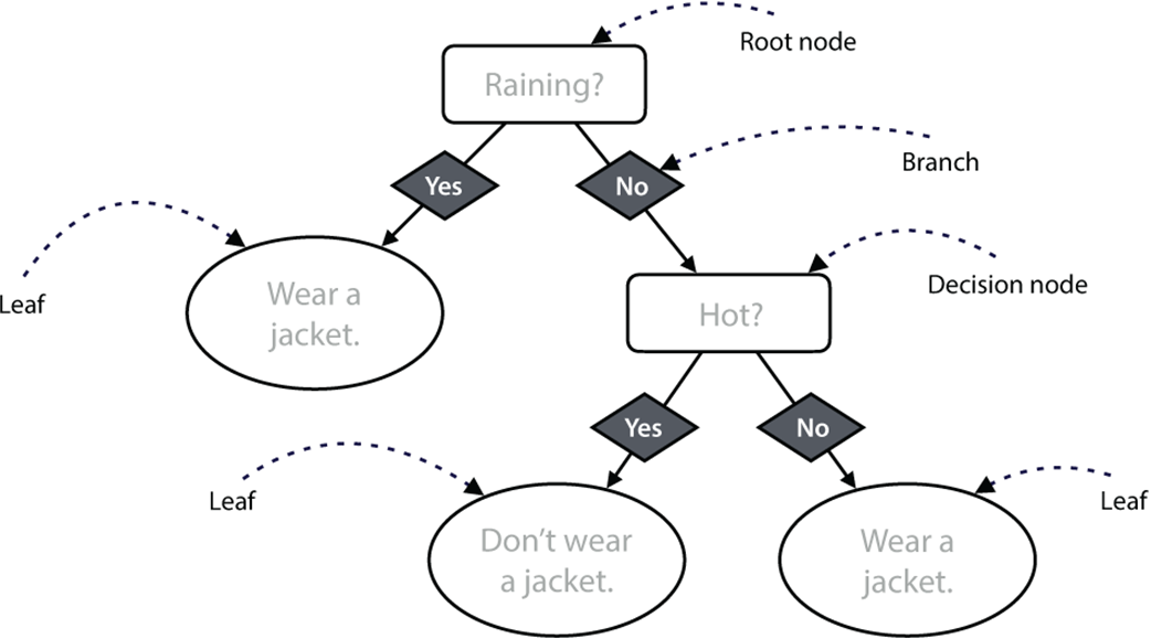
A regular decision tree with a root node, decision nodes, branches, and leaves. Note that each decision node contains a yes-or-no question. From each possible answer, one branch emanates, which can lead to another decision node or a leaf. This tree has a depth of 2, because the longest path from a leaf to the root goes through two branches.

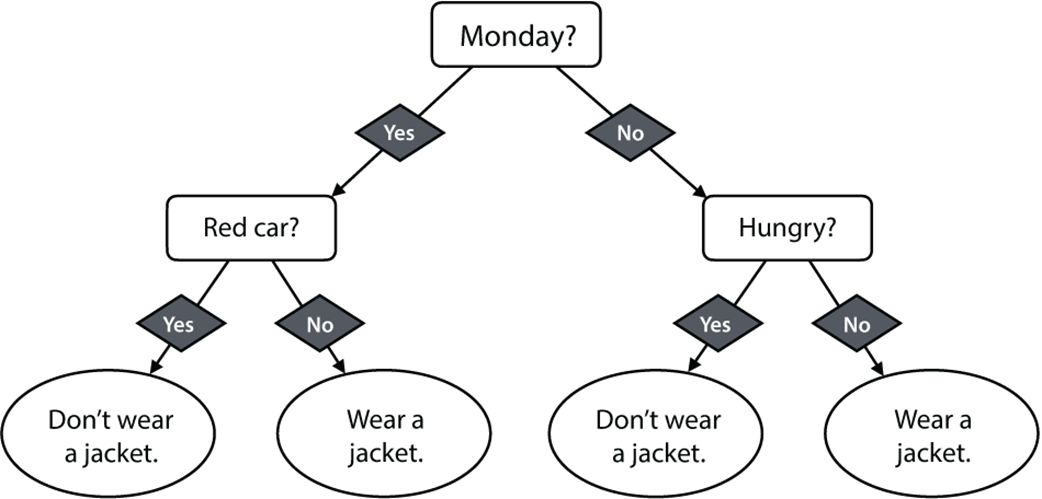
A second (maybe not as good) decision tree we could use to decide whether we want to wear a jacket on a given day

A simple decision tree (decision stump) that consists of only the question, “Is it raining?” If the answer is yes, the decision we make is to wear a jacket. If the answer is no, the decision we make is not to wear a jacket.

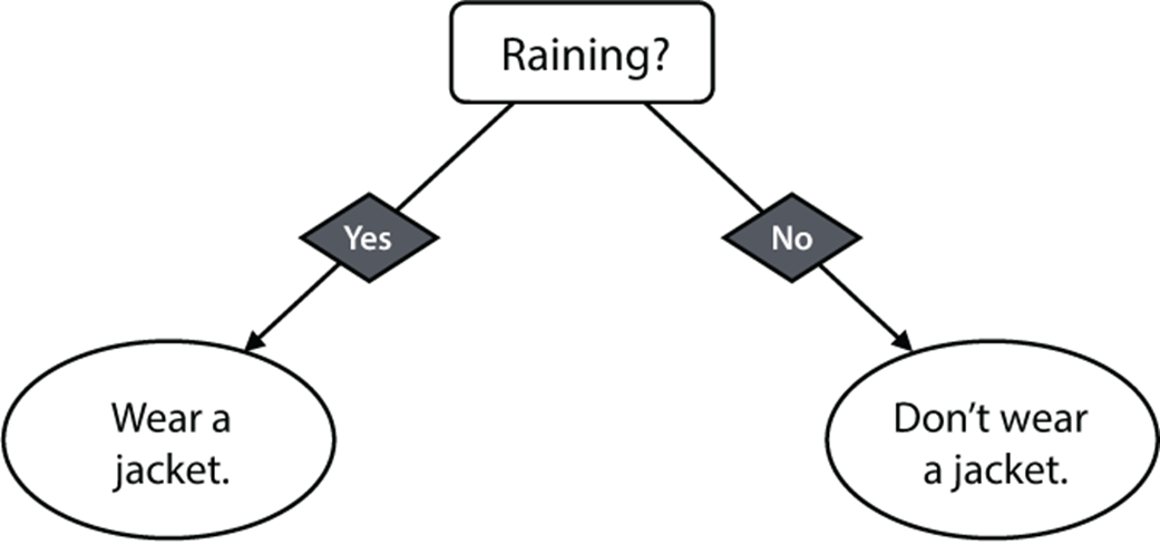
A slightly more complicated decision tree than the one in figure 9.4, where we have picked one leaf and split it into two further leaves. This is the same tree as in figure 9.1.

The three apps we are recommending: Atom Count, an app for counting the number of atoms in your body; Beehive Finder, an app for locating the nearest beehives to your location; and Check Mate Mate, an app for finding Australian chess players in your area

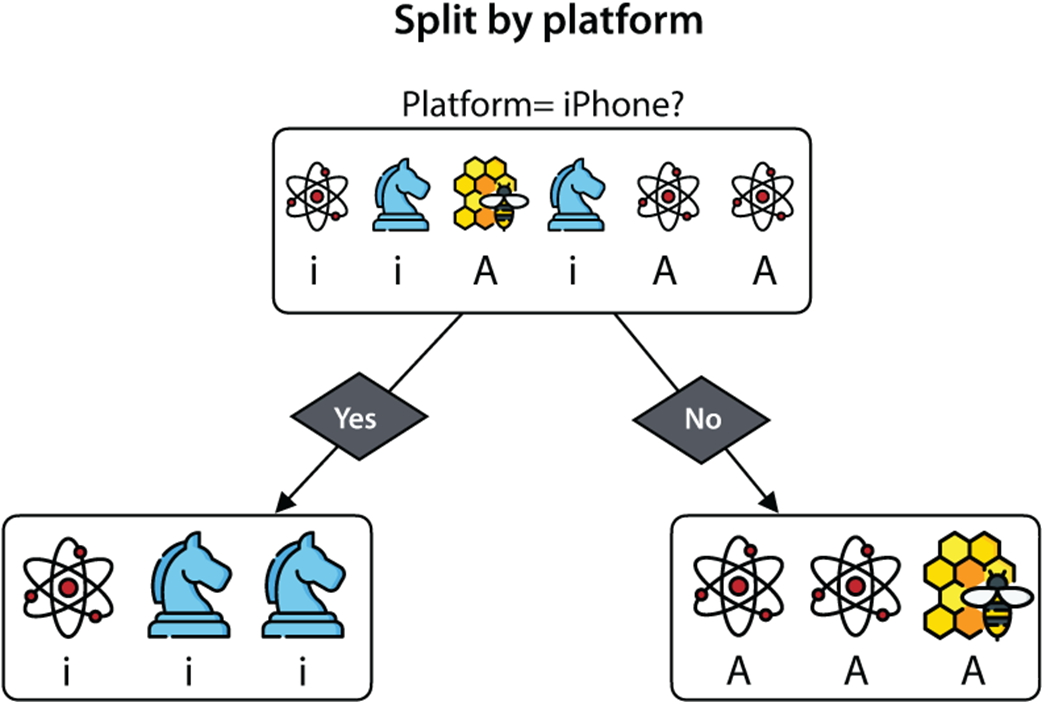
If we split our users by platform, we get this split: the iPhone users are on the left, and the Android users on the right. Of the iPhone users, one downloaded Atom Count and two downloaded Check Mate Mate. Of the Android users, two downloaded Atom Count and one downloaded Beehive Finder.

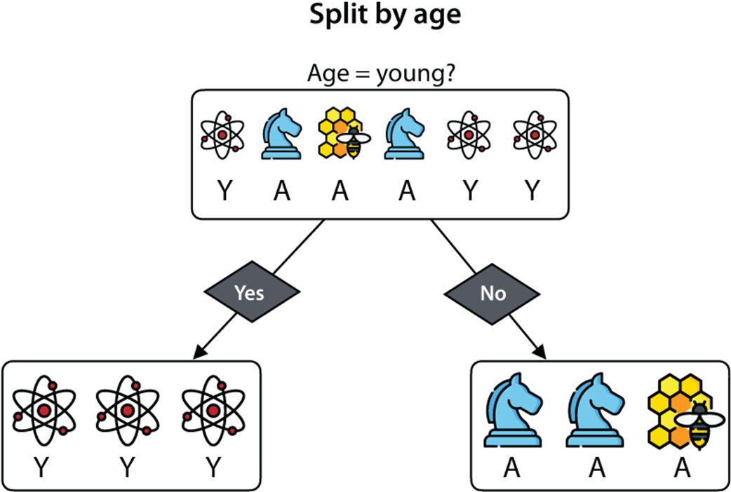
If we split our users by age, we get this split: the young are on the left, and the adults on the right. Out of the young users, all three downloaded Atom Count. Out of the adult users, one downloaded Beehive Finder and two downloaded Check Mate Mate.

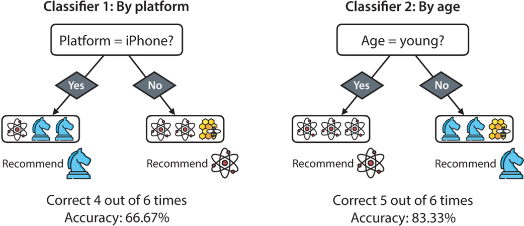
Classifier 1 uses platform, and classifier 2 uses age. To make the prediction at each leaf, each classifier picks the most common label among the samples in that leaf. Classifier 1 is correct four out of six times, and classifier 2 is correct five out of six times. Therefore, based on accuracy, classifier 2 is better.

Summary of the calculation of the Gini impurity index

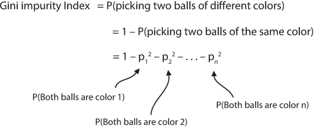
The calculation of the Gini index for the set with eight black balls and two white balls. Note that if the total area of the square is 1, the probability of picking two black balls is 0.82, and the probability of picking two white balls is 0.22 (these two are represented by the shaded squares). Thus, the probability of picking two balls of a different color is the remaining area, which is 1 – 0.82 – 0.22 =0.32. That is the Gini index.

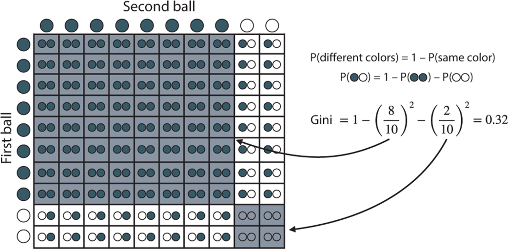
The two ways to split the dataset, by platform and age, and their Gini index calculations. Notice that splitting the dataset by age gives us two smaller datasets with a lower average Gini index. Therefore, we choose to split the dataset by age.

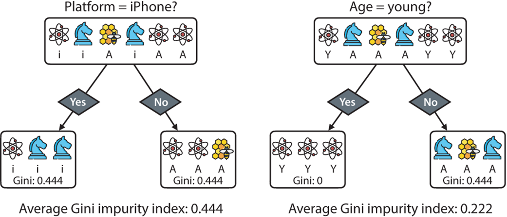
The two ways to split the dataset, by platform and age, and their entropy calculations. Notice that splitting the dataset by age gives us two smaller datasets with a lower average entropy. Therefore, we again choose to split the dataset by age.

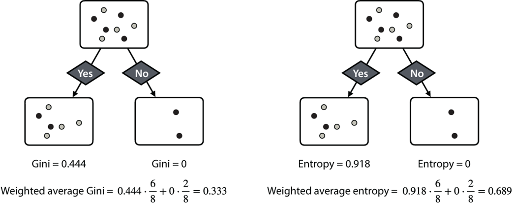
A split of a dataset of size eight into two datasets of sizes six and two. To calculate the average Gini index and the average entropy, we weight the index of the left dataset by 6/8 and that of the right dataset by 2/8. This results in a weighted Gini index of 0.333 and a weighted entropy of 0.689.

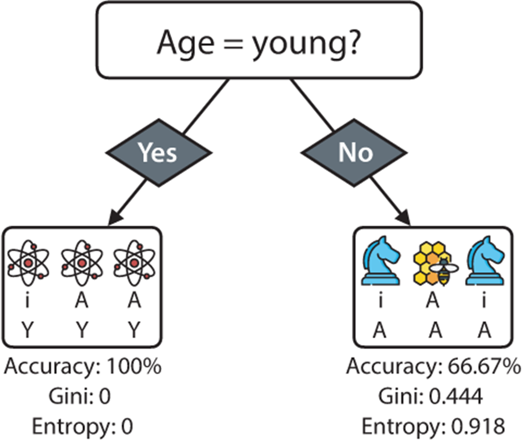
When we split our dataset by age, we get two datasets. The one on the left has three users who downloaded Atom Count, and the one on the right has one user who downloaded Beehive Count and two who downloaded Check Mate Mate.

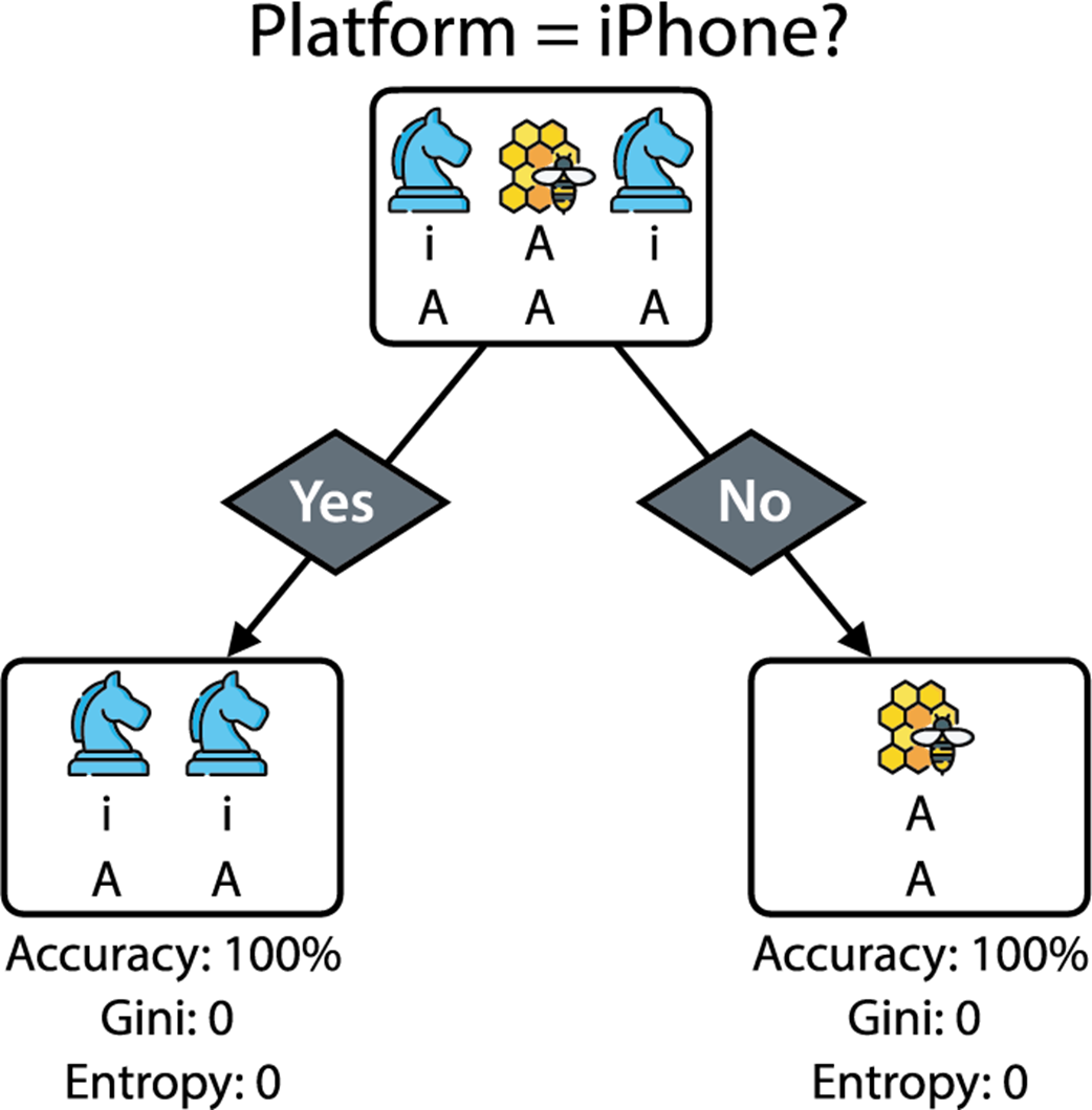
We can split the right leaf of the tree in figure 9.15 using platform and obtain two pure datasets. Each one of them has an accuracy of 100% and a Gini index and entropy of 0.

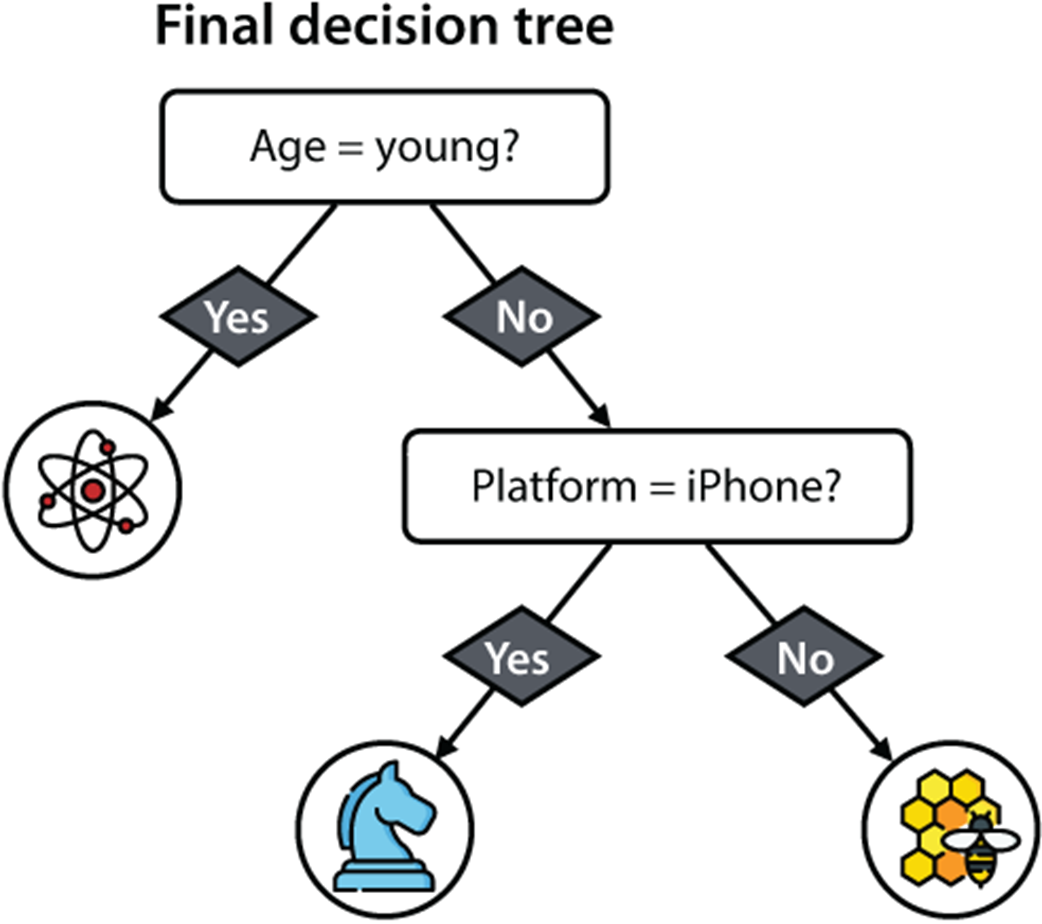
The resulting decision tree has two nodes and three leaves. This tree predicts every point in the original dataset correctly.

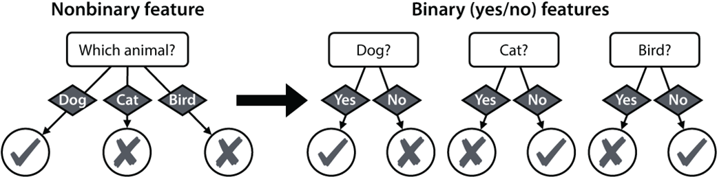
When we have a nonbinary feature, for example, one with three or more possible categories, we instead turn it into several binary (yes-or-no) features, one for each category. For example, if the feature is a dog, the answers to the three questions “Is it a dog?,” “Is it a cat?,” and “Is it a bird?” are “yes,” “no,” and “no.”

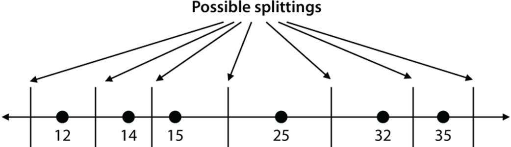
A graphic of the seven possible ways to split the users by age. Note that it doesn’t matter where we put the cutoffs, as long as they lie between consecutive ages (except for the first and last cutoff).

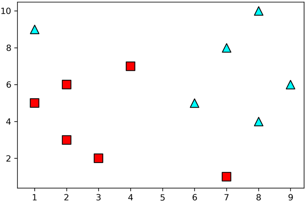
A dataset with two features (x0 and x1) and two labels (triangle and square) in which we will train a decision tree

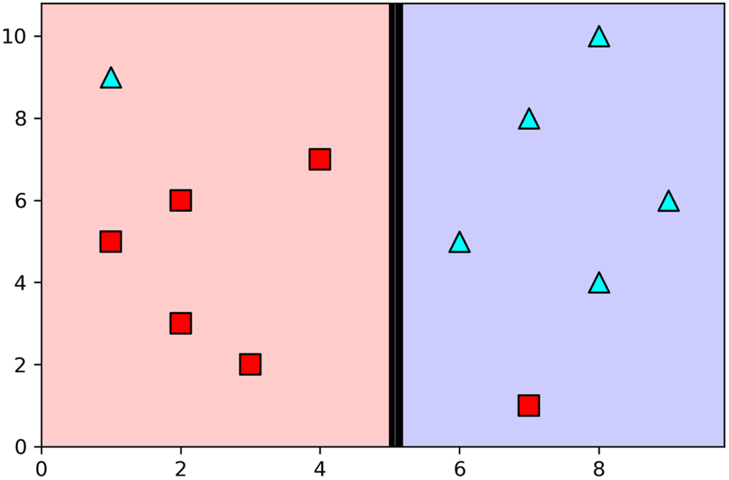
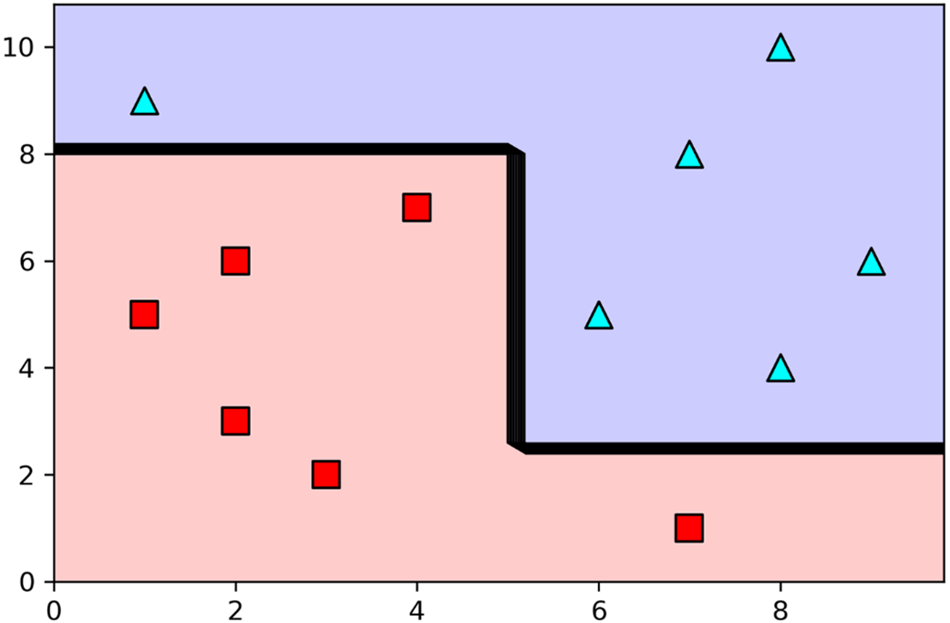
If we have to use only one vertical or horizontal line to classify this dataset in the best possible way, which one would we use? Based on accuracy, the best classifier is the vertical line at x0 = 5, where we classify everything to the right of it as a triangle, and everything to the left of it as a square. This simple classifier classifies 8 out of the 10 points correctly, for an accuracy of 0.8.

The classifier in figure 9.21 leaves us with two datasets, one at each side of the vertical line. If we had to classify each one of them, again using one vertical or horizontal line, which one would we choose? The best choices are horizontal lines at x1 = 8 and x1 = 2.5, as the figure shows.

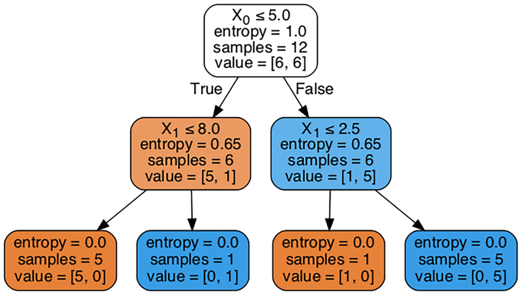
The resulting decision tree of depth 2 that corresponds to the boundary in figure 9.22. It has three nodes and four leaves.

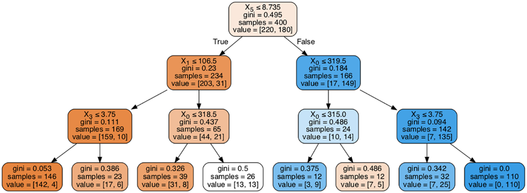
A decision tree of depth 3 trained in the student admissions dataset

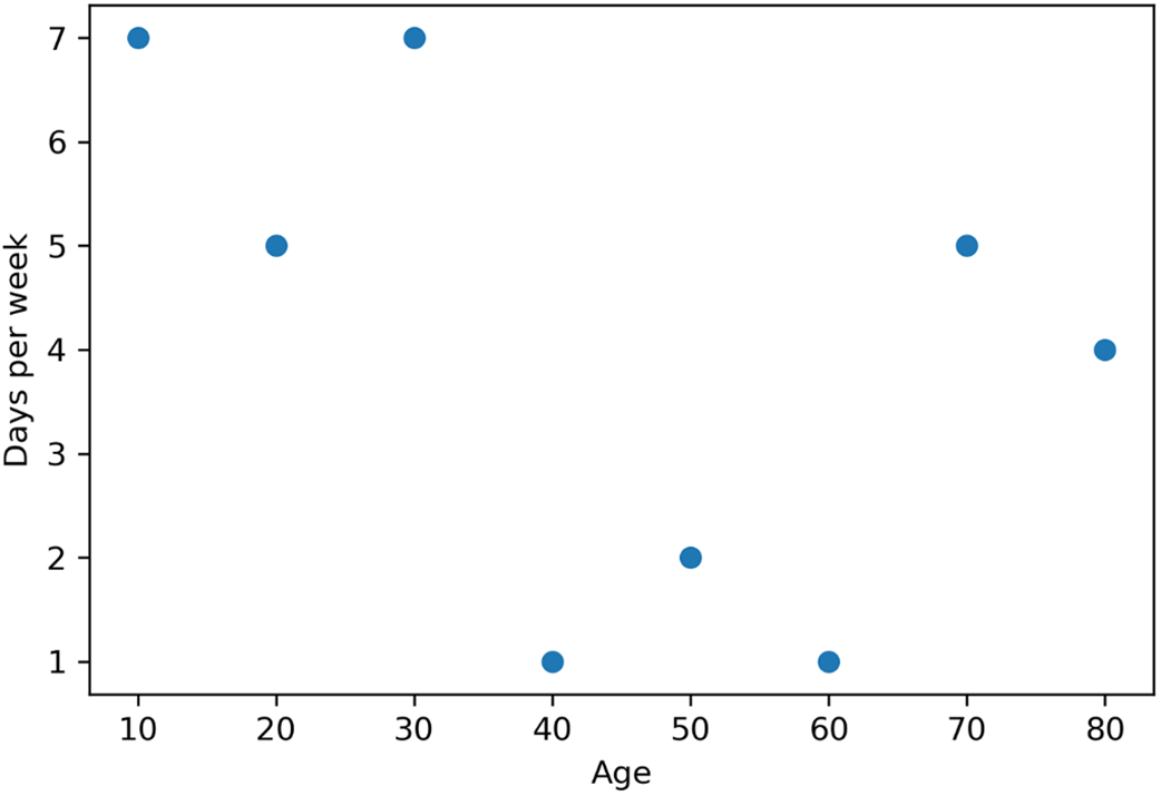
The plot of the dataset in table 9.6, where the horizontal axis corresponds to the age of the user and the vertical axis to the number of days per week that they engaged with the app

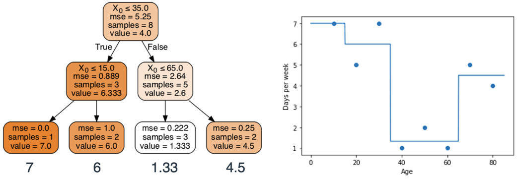
Left: The resulting decision tree obtained in Scikit-Learn. This tree has three decision nodes and four leaves. Right: The plot of the predictions made by this decision tree. Note that the cutoffs are at ages 35, 15, and 65, corresponding to the decision nodes in the tree. The predictions are 7, 6, 1.33, and 4.5, corresponding to the leaves in the tree.

FAQ