8 Using probability to its maximum: The naive Bayes model

This chapter introduces Bayes’ theorem as a practical way to turn partial information into calibrated probabilities. It explains the flow from a prior (an initial, context-free belief) to an event that provides evidence, and finally to a posterior—an updated belief that incorporates that evidence. Through intuitive stories (like guessing an animal or interpreting a medical test for a rare disease), the text shows why raw accuracy can be misleading when base rates are tiny, and how conditional probability, the product rule, and normalization combine to yield Bayes’ formula. Tree diagrams and simple counts make the math tangible and highlight how to partition outcomes, compute intersections, and normalize to get probabilities that add to one.

With these foundations, the chapter builds a spam‑detection case study. First, it estimates a prior spam rate from a labeled inbox. Then, using evidence such as the presence of a word (for example, “lottery”), it computes P(word | class) from counts and normalizes to obtain P(class | word). To handle multiple words, it adopts the “naive” independence assumption—treating word appearances as conditionally independent given the class—so the joint likelihood becomes a simple product across words. Despite being an approximation, this yields a fast, effective classifier that produces meaningful probabilities; the examples show how combining signal words can push the posterior near 1 for spam or keep it low for ham, and how new evidence can raise or lower the estimate in an interpretable way.

The implementation section walks through turning raw emails into lowercase, deduplicated word sets; counting word occurrences separately for spam and ham; and converting counts to conditional probabilities. It highlights two pragmatic tricks: additive smoothing (initializing counts at 1 to avoid zero probabilities) and rescaling products to prevent numerical underflow, followed by a final normalization to return a probability in [0, 1]. A simple predictor multiplies the per‑word likelihoods with the prior and compares the result across classes. The chapter closes by noting strengths (speed, simplicity, interpretability) and limits (the independence assumption, basic bag‑of‑words features), and points to straightforward extensions such as better smoothing, richer text preprocessing, and production‑grade library implementations for larger datasets.

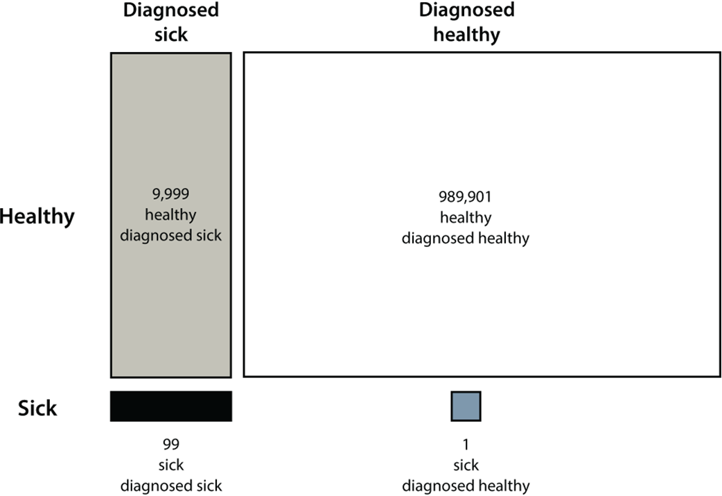
Among our 1,000,000 patients, only 100 of them are sick (bottom row). Among the 10,098 diagnosed as sick (left column), only 99 of them are actually sick. The remaining 9,999 are healthy, yet were misdiagnosed as sick. Therefore, if our friend was diagnosed as sick, he has a much higher chance to be among the 9,999 healthy (top left) than to be among the 99 sick (bottom left).

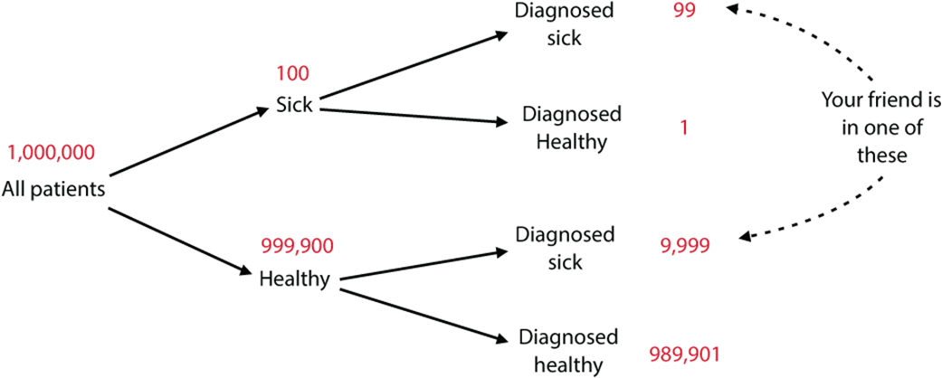
The tree of possibilities. Each patient can be sick or healthy. For each of the possibilities, the patient can be diagnosed as sick or healthy, which gives us four possibilities. We start with one million patients: 100 of them are sick, and the remaining 999,900 are healthy. Out of the 100 sick, one gets misdiagnosed as healthy, and the remaining 99 get correctly diagnosed as sick. Out of the 999,900 healthy patients, 9,999 get misdiagnosed as sick, and the remaining 989,901 are correctly diagnosed as healthy.

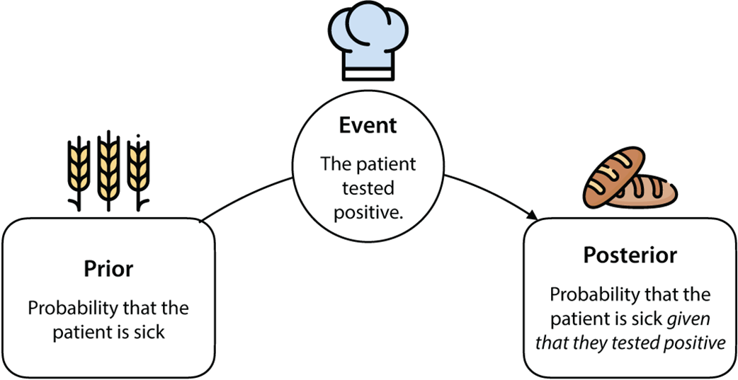
The prior, the event, and the posterior. The prior is the “raw” probability, namely, the probability we calculate when we know very little. The event is the information that we obtain, which will help us refine our calculation of the probability. The posterior is the “cooked” probability, or the much more accurate probability that we calculate when we have more information.

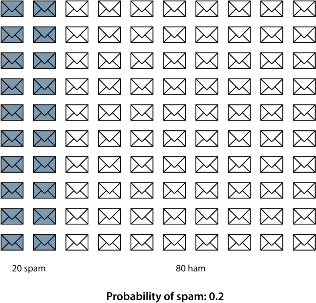
We have a dataset with 100 emails, 20 of which are spam. An estimate for the probability that an email is spam is 0.2. This is the prior probability.

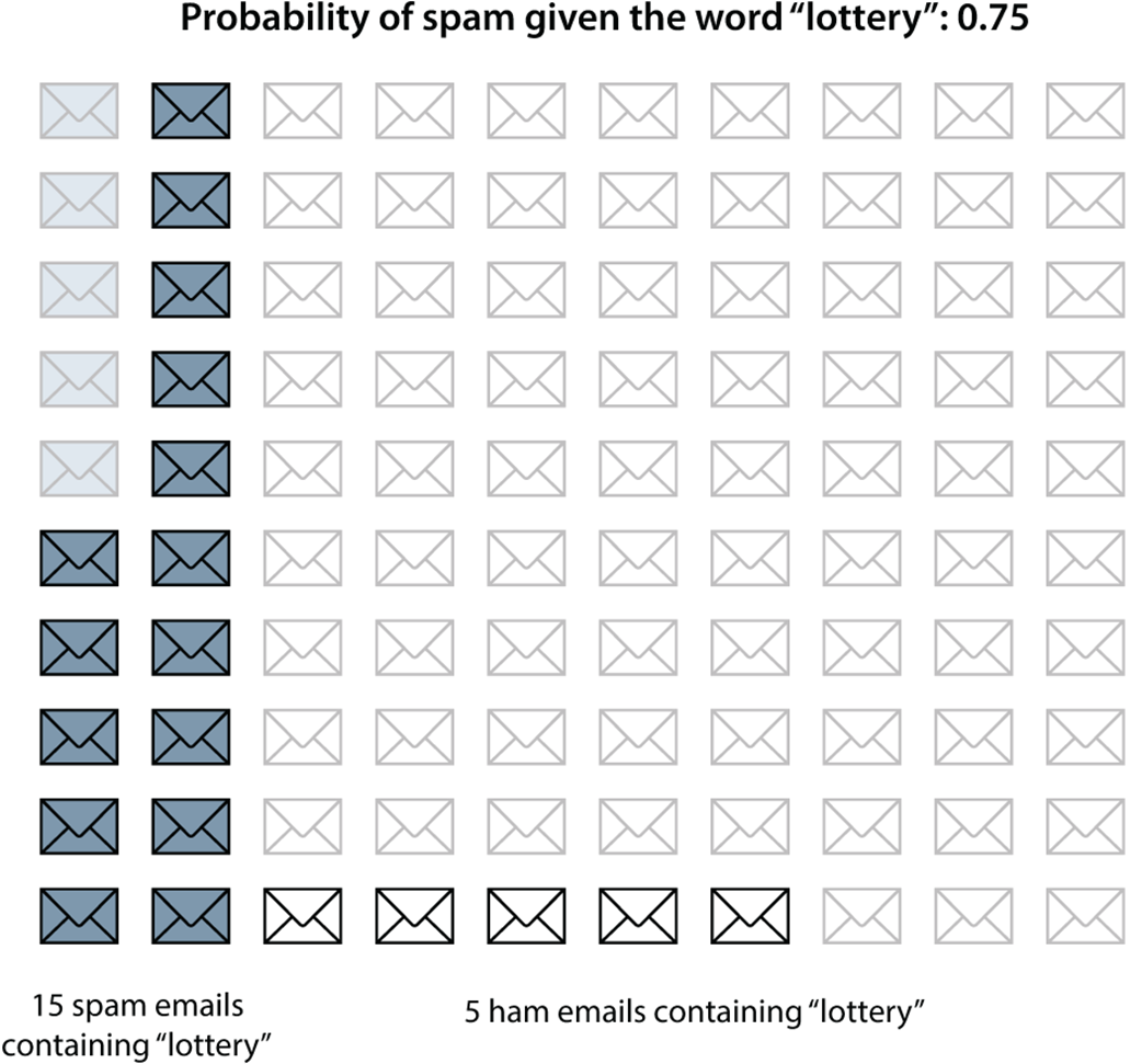
We have removed (grayed out) the emails that don’t contain the word lottery. All of a sudden, our probabilities change. Among the emails that contain the word lottery, there are 15 spam emails and 5 ham emails, so the probability that an email containing the word lottery is spam, is 15/20 = 0.75.

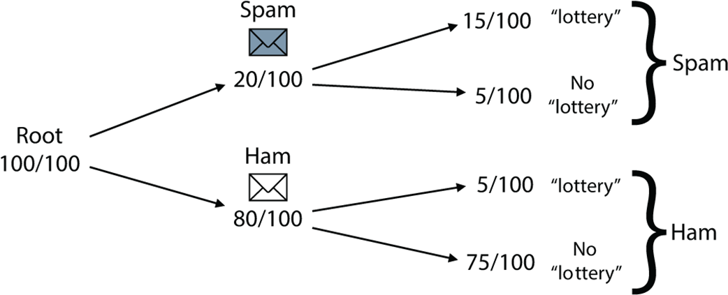
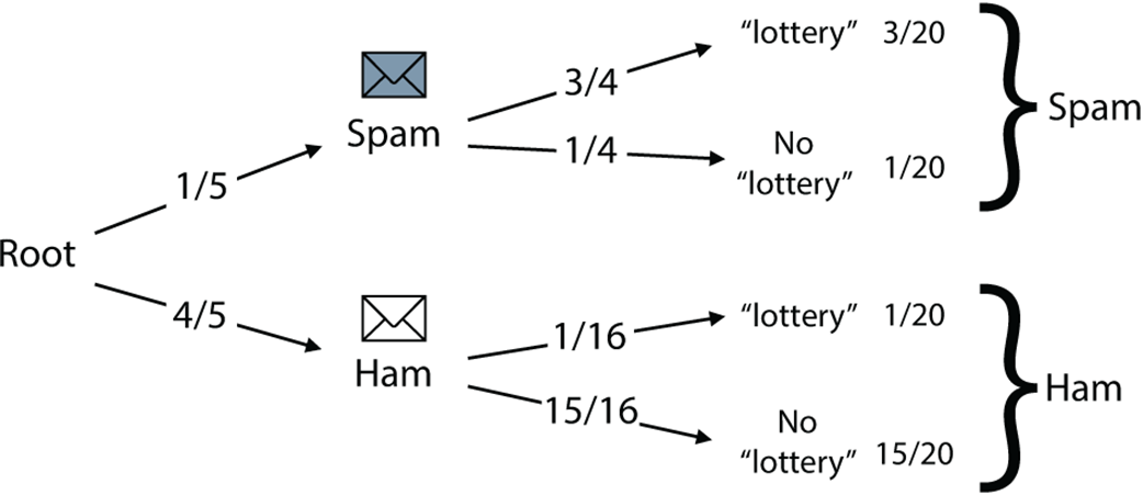
The tree of possibilities. The root splits into two branches: spam and ham. Then each of these splits into two branches: when the email contains the word lottery, and when it doesn’t.

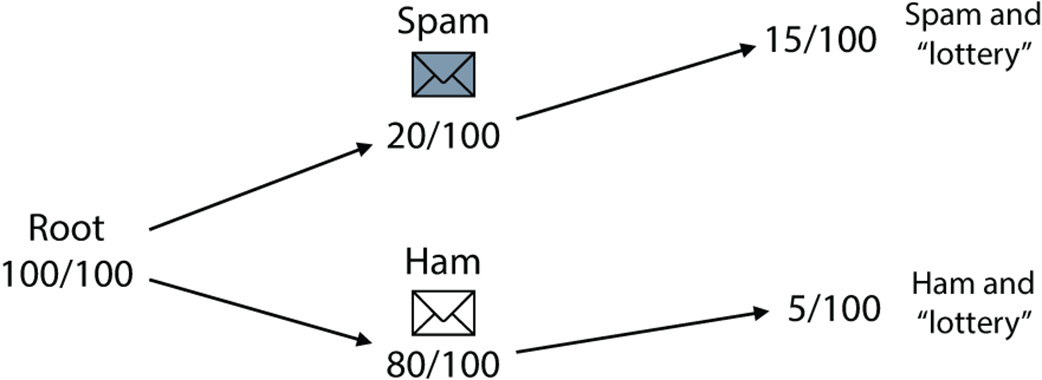
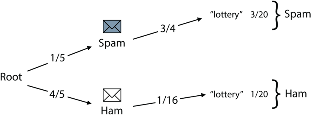
From the previous tree, we have removed the two branches where the emails don’t contain the word lottery. Out of the original 100 emails, we have 20 left that contain lottery. Because of these 20 emails, 15 are spam, we conclude that the probability that an email is spam given that it contains the word lottery is 0.75.

The same tree from figure 8.6, but now with probabilities. From the root, two branches emerge, one for spam emails and one for ham emails. In each one, we record the corresponding probability. Each branch again splits into two leaves: one for emails containing the word lottery, and one for emails not containing it. In each branch we record the corresponding probability. Notice that the product of these probabilities is the probability at the right of each leaf. For example, for the top leaf, 1/5 3/4 = 3/20 = 0.15.

From the tree in figure 8.8, we have removed the two branches where the emails don’t contain the word lottery.

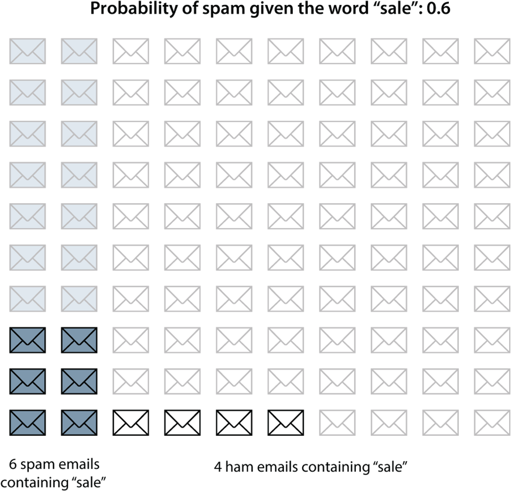
In a similar calculation as for the word lottery, we look at the emails containing the word sale. Among these (not grayed-out) emails, there are six spam and four ham.

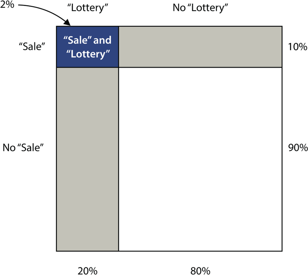
Say 20% of the emails contain the word lottery, and 10% of the emails contain the word sale. We make the naive assumption that these two words are independent of each other. Under this assumption, the percentage of emails that contain both words can be estimated as 2%, namely, the product of 20% and 10%.

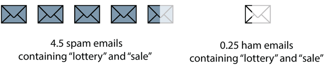
We have 4.5 spam emails and 0.25 ham emails. We throw a dart, and it hits one of the emails. What is the probability that it hit a spam email? The answer is 94.74%.

FAQ