Overview

6 A continuous approach to splitting points: Logistic classifiers

This chapter replaces hard, yes/no decisions with soft, probabilistic ones by introducing logistic classifiers—a continuous version of perceptrons that output scores between 0 and 1. A linear score from the input features is passed through the sigmoid function to produce a probability that can be interpreted as confidence in a class (for instance, the likelihood a sentence is “happy”). A 0.5 threshold can still yield a binary decision, but the probability itself carries richer information. The chapter motivates this continuous view with intuitive examples, shows how it supports evaluation and decision-making, and previews practical uses such as sentiment analysis and the extension to multiple classes via the softmax function.

To measure how well a logistic classifier fits data, the chapter evaluates several error functions and lands on log loss (cross-entropy) as the preferred choice. Absolute and square errors behave sensibly but are bounded and less aligned with probability theory. Log loss, derived from the negative log-likelihood of the observed labels, adds across examples, penalizes overconfident mistakes more severely, and makes it easy to compare models: lower total log loss indicates a better classifier. Conceptually, it asks the model to assign high probability to the true label of each point, converting products of probabilities into sums of logarithms for numerical stability and analytical convenience.

Training proceeds via the logistic regression algorithm, a gradient-descent procedure that repeatedly applies the “logistic trick.” Concretely, weights and bias are nudged by the term (y − ŷ) scaled by the feature values and a learning rate, which has an intuitive geometric effect: move the decision boundary closer to misclassified points and farther from correctly classified ones. The approach generalizes to many features and is typically implemented with stochastic or mini-batch updates; coding it by hand shows the log loss steadily decreasing, while a scikit-learn pipeline demonstrates a real application on IMDB movie reviews using bag-of-words features. Finally, the chapter introduces softmax to handle more than two classes by exponentiating class scores and normalizing them into a coherent probability distribution (which reduces to the sigmoid in the binary case).

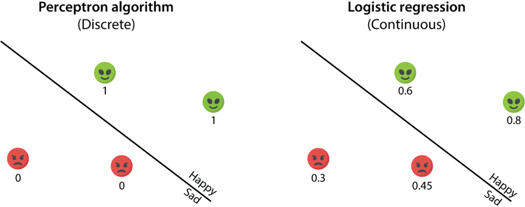
Left: The perceptron algorithm trains a discrete perceptron, where the predictions are 0 (happy) and 1 (sad). Right: The logistic regression algorithm trains a continuous perceptron, where the predictions are numbers between 0 and 1 which indicate the predicted level of happiness.

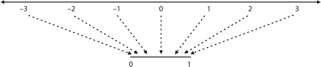
The sigmoid function sends the entire number line to the interval (0,1).

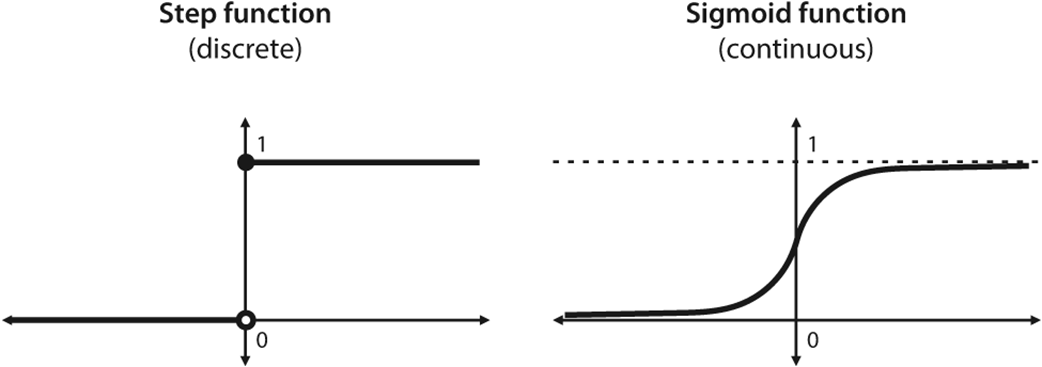
Left: The step function used to build discrete perceptrons. It outputs a value of 0 for any negative input and a value of 1 for any input that is positive or zero. It has a discontinuity at zero. Right: The sigmoid function used to build continuous perceptrons. It outputs values less than 0.5 for negative inputs and values greater than 0.5 for positive inputs. At zero, it outputs 0.5. It is continuous and differentiable everywhere.

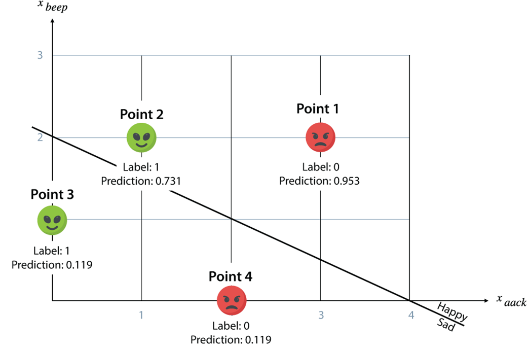
The plot of the dataset in table 6.2 with predictions. Notice that points 2 and 4 are correctly classified, but points 1 and 3 are misclassified.

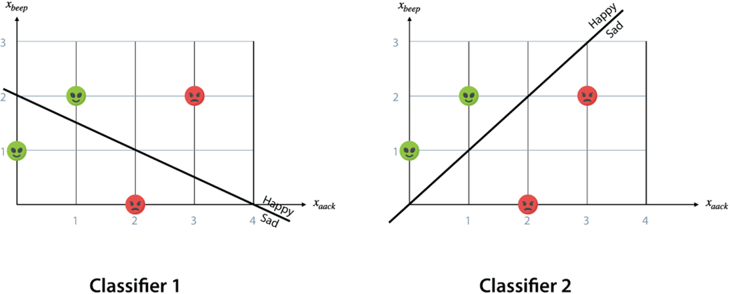
Left: A bad classifier that makes two mistakes. Right: A good classifier that classifies all four points correctly.

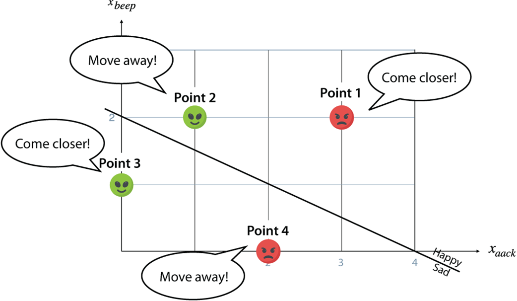
In the logistic regression algorithm, every point has a say. Points that are correctly classified tell the line to move farther away, to be deeper in the correct zone. Points that are incorrectly classified tell the line to come closer, in hopes of one day being on the correct side of the line.

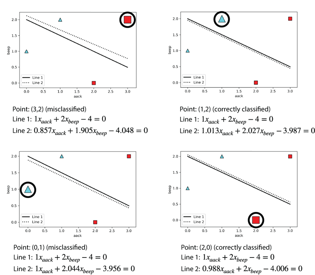
The logistic trick applied to each of the four data points. Notice that for correctly classified points, the line moves away from the point, whereas for misclassified points, the line moves closer to the point.

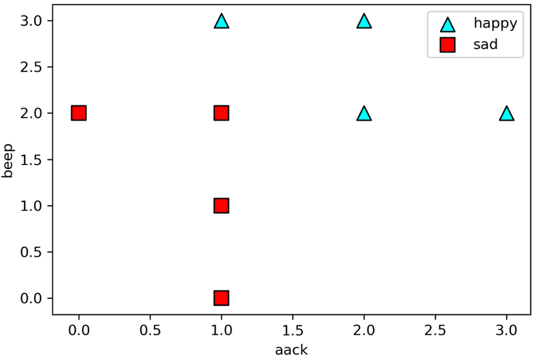
The plot of our dataset, where the happy sentences are represented by triangles and the sad sentences by squares.

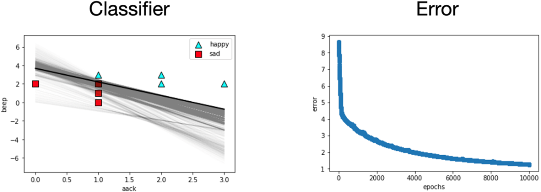
Left: The plot of the resulting classifier, and the intermediate steps. Right: The error plot. Notice that the more epochs we run the logistic regression algorithm, the lower the error gets.

FAQ

What is a logistic classifier and how does it differ from a (discrete) perceptron?

A logistic classifier is a “continuous perceptron” that outputs a number between 0 and 1 for each input, interpreted as the probability of class 1. A discrete perceptron uses a step function and returns only 0 or 1. Logistic classifiers use the sigmoid activation, so they provide graded confidence rather than a hard yes/no.

Why is the model called logistic regression if it’s used for classification?

The algorithm that trains a logistic classifier is historically called logistic regression because it fits parameters by regressing a linear score through a logistic (sigmoid) link. Although the output is a probability and we make a classification by thresholding, the training procedure and the functional form gave rise to the “regression” name.

What is the sigmoid function and why is it preferred over the step function?

The sigmoid s(x) maps any real number to (0, 1), is continuous and differentiable everywhere, and produces values near 0 for large negative inputs, near 1 for large positive inputs, and 0.5 at 0. Unlike the step function, it has a useful derivative, enabling gradient-based optimization and providing probabilistic scores instead of hard labels.

How should I interpret the output of a logistic classifier and choose a decision threshold?

The output ŷ in [0,1] is the estimated probability that the input belongs to class 1. A common default threshold is 0.5: predict class 1 if ŷ ≥ 0.5, else class 0. This threshold is arbitrary; you can move it to trade off precision and recall or optimize a metric that matters for your task.

Which error (loss) functions can be used, and why is log loss preferred?

Absolute error and squared error both measure distance between label and prediction but stay small (≤1) and are less convenient for optimization. Log loss (negative log-likelihood) directly scores how much probability the model assigns to the true label, penalizing confident wrong predictions heavily and working nicely with gradient descent. It also sums cleanly across examples.

What is the formula for log loss and how does it behave?

For a single labeled example with label y ∈ {0,1} and prediction ŷ: log_loss = −[ y·ln(ŷ) + (1−y)·ln(1−ŷ) ]. If the model assigns high probability to the correct label, the loss is small; if it assigns low probability, the loss is large. The dataset loss is the sum (or mean) over all examples.

What is the “logistic trick” and how does it update the model?

The logistic trick is the per-example update derived from gradient descent on log loss. For features x = (x1, x2, …), weights w = (w1, w2, …), bias b, prediction ŷ = s(w·x + b), and learning rate h: wi ← wi + h·(y − ŷ)·xi for each i, and b ← b + h·(y − ŷ). Intuitively, if a point is misclassified, the boundary moves closer; if it’s correctly classified, it moves slightly farther, increasing confidence.

How does the logistic regression training loop work (SGD, mini-batch, batch)?

Start with random weights and bias. Repeat for many epochs: pick data (a single example for SGD, a small set for mini-batch, or the whole dataset for batch), compute predictions, compute the gradient of log loss, and update parameters using the logistic trick. Monitor log loss to judge convergence. Mini-batch is typically the practical default.

How do I build a logistic classifier from scratch and with scikit-learn?

From scratch: implement sigmoid, a scoring function (dot product + bias), the prediction ŷ = s(score), log loss, and the update rule wi ← wi + h·(y − ŷ)·xi; b ← b + h·(y − ŷ). Loop over epochs using SGD or mini-batches. With scikit-learn: vectorize inputs (e.g., CountVectorizer for text), map labels to {0,1}, then fit a LogisticRegression model. Use predict_proba for probabilities and inspect coefficients to see influential features.

How do we handle more than two classes with logistic models?

Use one linear score per class and apply the softmax function to convert scores into a probability distribution across all classes. For class i with score ai, pi = exp(ai) / Σj exp(aj). The predicted class is the one with the highest probability. With two classes, softmax reduces to the sigmoid.

Left: The perceptron algorithm trains a discrete perceptron, where the predictions are 0 (happy) and 1 (sad). Right: The logistic regression algorithm trains a continuous perceptron, where the predictions are numbers between 0 and 1 which indicate the predicted level of happiness.

The sigmoid function sends the entire number line to the interval (0,1).

The plot of the dataset in table 6.2 with predictions. Notice that points 2 and 4 are correctly classified, but points 1 and 3 are misclassified.

Left: A bad classifier that makes two mistakes. Right: A good classifier that classifies all four points correctly.

In the logistic regression algorithm, every point has a say. Points that are correctly classified tell the line to move farther away, to be deeper in the correct zone. Points that are incorrectly classified tell the line to come closer, in hopes of one day being on the correct side of the line.

The logistic trick applied to each of the four data points. Notice that for correctly classified points, the line moves away from the point, whereas for misclassified points, the line moves closer to the point.

The plot of our dataset, where the happy sentences are represented by triangles and the sad sentences by squares.

Left: The plot of the resulting classifier, and the intermediate steps. Right: The error plot. Notice that the more epochs we run the logistic regression algorithm, the lower the error gets.

pro $24.99 per month

lite $19.99 per month

team

pro

team

pro

team