Overview

5 Using lines to split our points: The perceptron algorithm

This chapter introduces classification as the task of predicting categories rather than numbers and uses sentiment analysis to ground the ideas. The perceptron is presented as a simple linear classifier that assigns a weight to each feature and adds a bias; its decision is made by applying a step function to the resulting score. Geometrically, in two features it draws a line that splits the plane into a positive and a negative region; with more features the boundary becomes a hyperplane. Through toy alien-language examples, the chapter shows how word counts become features, how a bias behaves like a threshold, and why perfect separation is not always possible (for instance, when word order or sarcasm changes meaning without changing counts).

Training a perceptron follows the perceptron algorithm: start with random weights and bias, then repeatedly improve them with the perceptron trick. Each misclassified point nudges the boundary slightly toward itself by updating weights and bias in proportion to the learning rate and the point’s features; correctly classified points leave the model unchanged. To measure progress, the chapter develops the mean perceptron error: for misclassified points, use the absolute value of the score (a simple surrogate for distance to the boundary), and average across the dataset. This error guides gradient-descent style learning, and the chapter contrasts naive mistake counting (too coarse) and true geometric distance (costly) with the practical score-based error. It also outlines stochastic, mini-batch, and batch updates, and explains key hyperparameters such as learning rate and epochs.

Practically, the chapter codes the algorithm from scratch (score, step, prediction, error, update step, and training loop) and then shows how to use a ready-made Perceptron in scikit-learn. It interprets parameters (weights reflect feature “happiness/sadness,” the bias captures the inherent label of an “empty” input), generalizes from lines to planes in higher dimensions, and demonstrates which logical gates are linearly separable (AND/OR) and which are not (XOR). The chapter closes with applications—spam filtering, recommendation systems, health diagnostics, and computer vision—and positions the perceptron as both a serviceable linear classifier and a foundational building block for more powerful models such as logistic regression and neural networks.

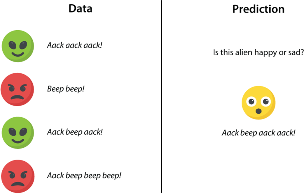
Our dataset of aliens. We have recorded their mood (happy or sad) and the sentence they keep repeating. Now a fifth alien comes in, saying a different sentence. Do we predict that this alien is happy or sad?

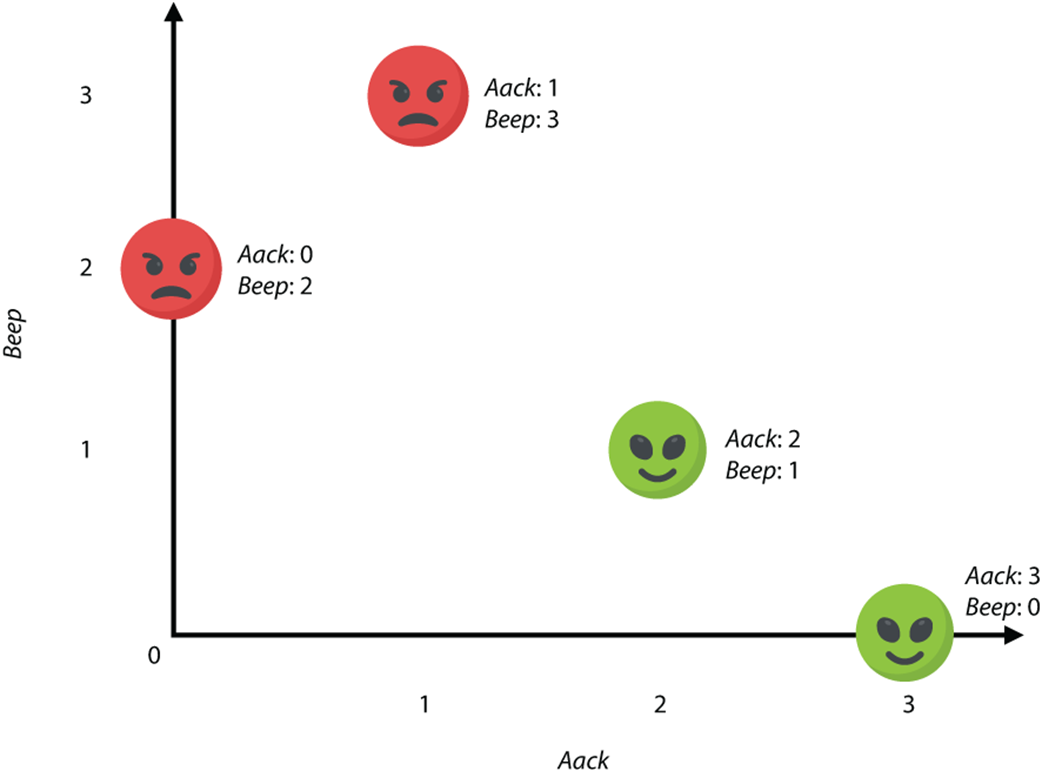
A plot of the dataset of aliens. In the horizontal axis we plot the number of appearances of the word aack, and in the vertical axis, the appearances of the word beep.

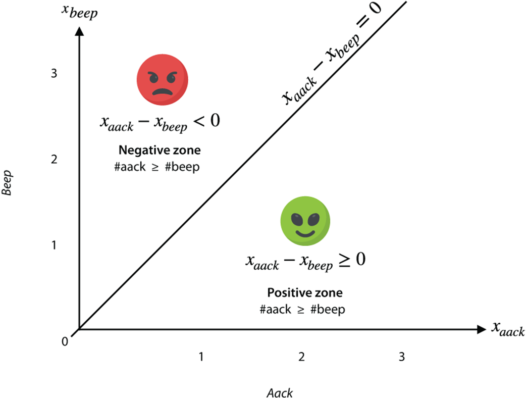
The classifier is the diagonal line that splits the happy and the sad points. The equation of this line is xaack = xbeep (or equivalently, xaack – xbeep = 0), because the line corresponds to all the points where the horizontal and the vertical coordinates are equal. The happy zone is the zone in which the number of appearances of aack is greater than or equal to the number of appearances of beep, and the sad zone is the zone in which the number of appearances of aack is less than that of beep.

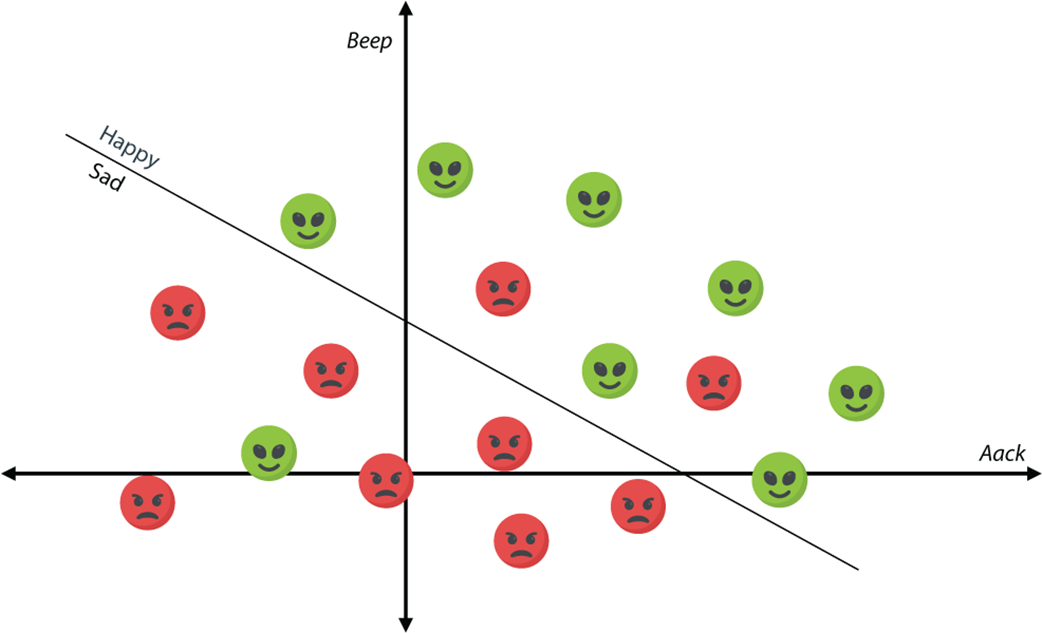
The plot of the new dataset of aliens. Notice that the happy ones tend to be above and to the right, and the sad ones below and to the left.

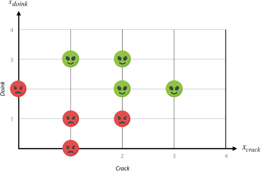
The classifier for the new dataset of aliens. It is again a line that splits the happy and the sad aliens.

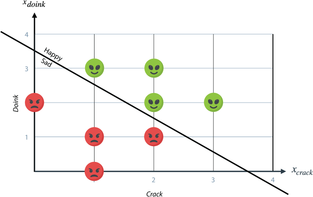
This line splits the dataset well. Note that it makes only three mistakes: two on the happy zone and one on the sad zone.

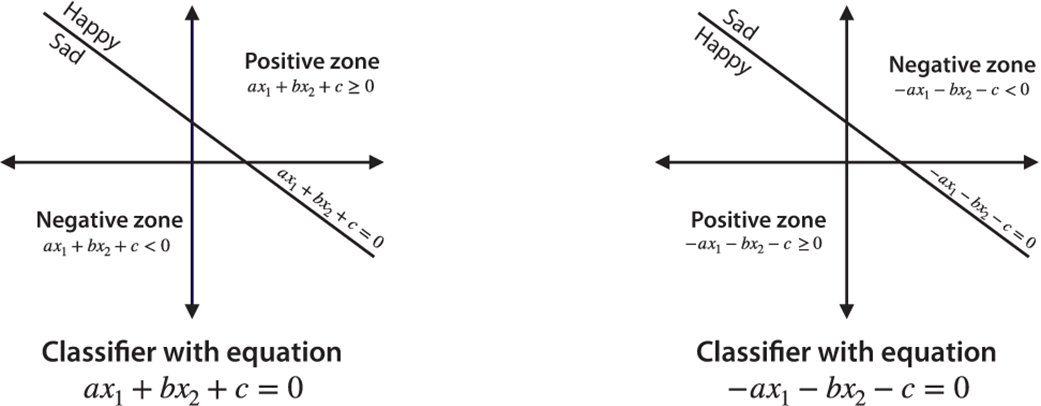
A classifier is defined by a line with the equation ax1 + bx2 + c = 0, a positive zone, and a negative zone. If we want to flip the positive and negative zones, all we need to do is negate the weights and the bias. On the left we have the classifier with equation ax1 + bx2 + c = 0. On the right, the classifier with flipped zones and the equation –ax1 – bx2 – c = 0.

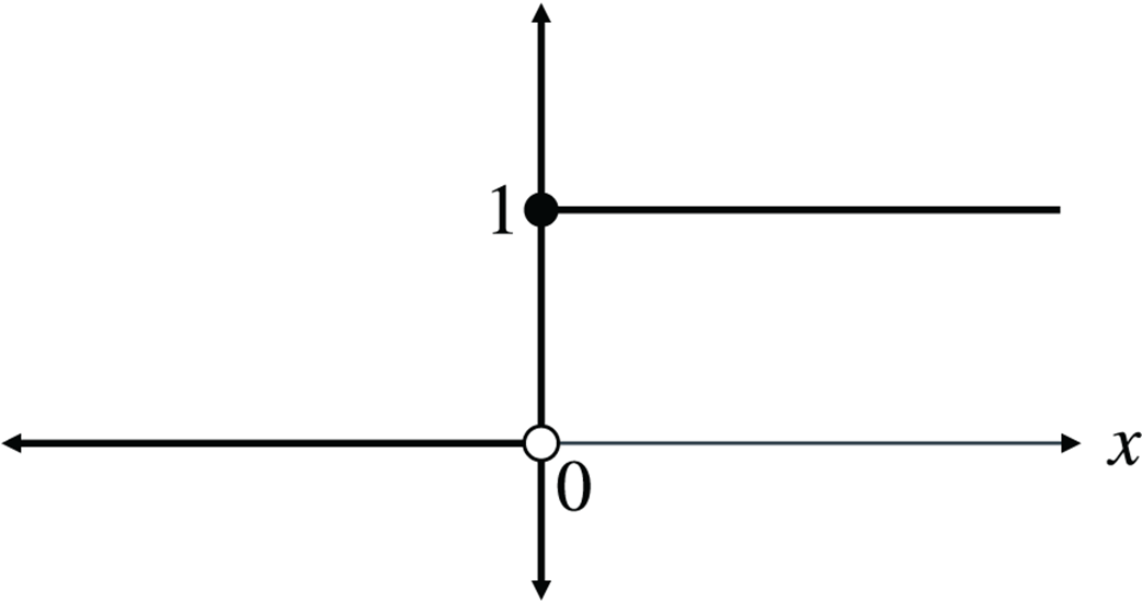
The step function is useful in the study of perceptron models. The output of the step function is 0 when the input is negative and 1 otherwise.

A sentence with three words can be plotted as a point in space. In this case, a sentence with the word aack five times, beep eight times, and crack three times is plotted in the point with coordinates (5,8,3).

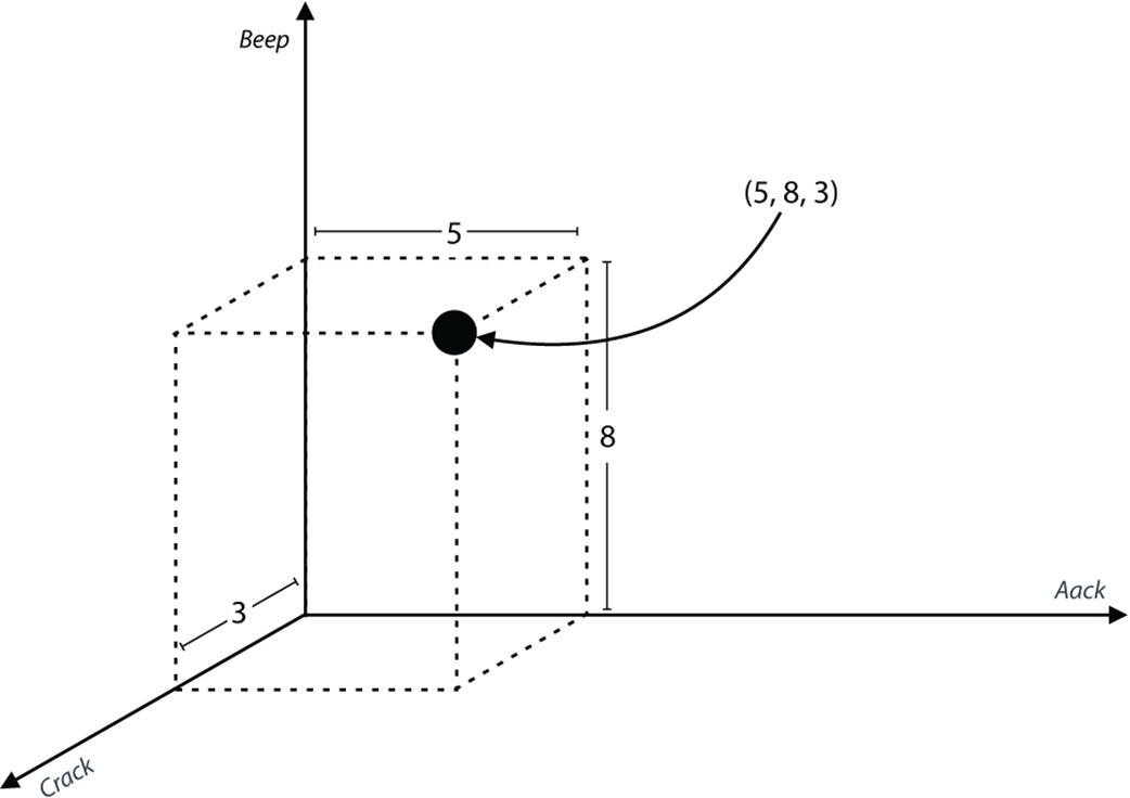
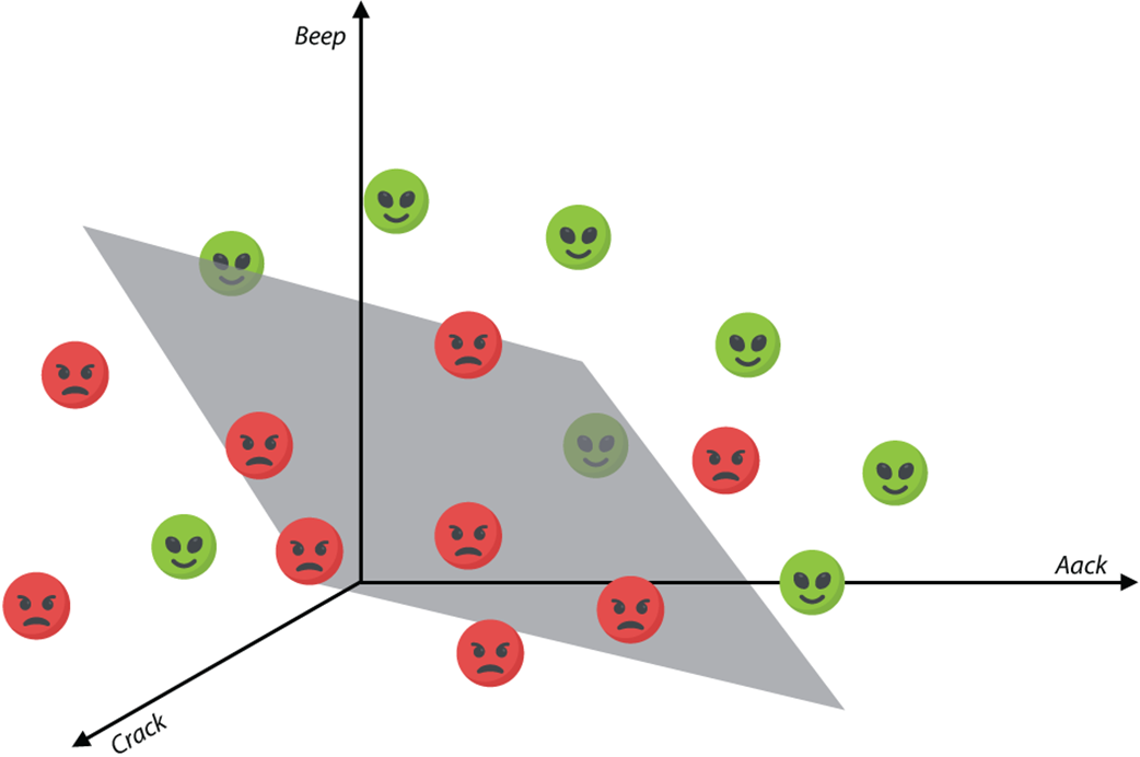
A dataset of sentences with three words is plotted in three dimensions. The classifier is represented by a plane that splits the space into two regions.

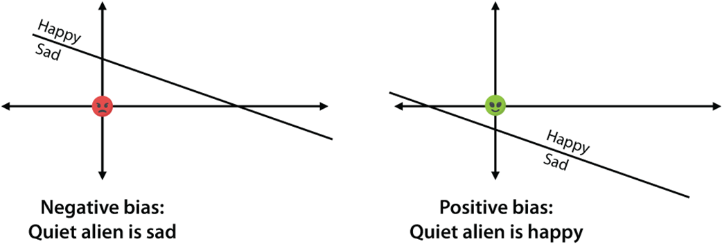
Left: the classifier has a negative bias, or a positive threshold (y-intercept). This means that the alien that doesn’t say anything falls in the sad zone and is classified as sad. Right: The classifier has a positive bias, or a negative threshold. This means that the alien that doesn’t say anything falls in the happy zone and is classified as happy.

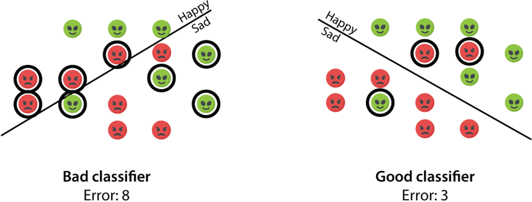
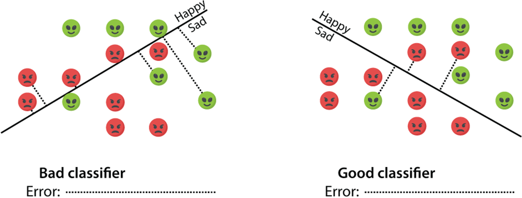
Left: a bad classifier, which doesn’t really split the points well. Right: a good classifier. Can we think of an error function that assigns a high number to the bad classifier and a low number to the good one?

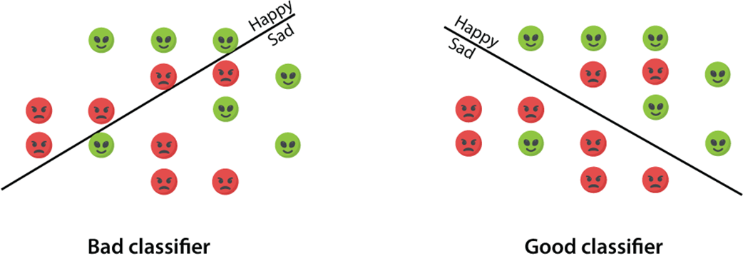
We evaluate the two classifiers by counting the number of points that each one of them misclassifies. The classifier on the left misclassifies eight points, whereas the classifier on the right misclassifies three points. Thus, we conclude that the classifier on the right is a better one for our dataset.

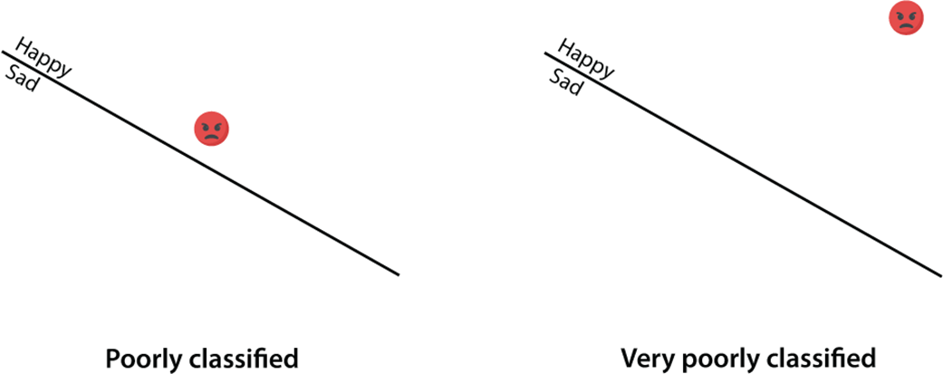
The two classifiers misclassify the point. However, the classifier on the right made a much bigger mistake than the classifier on the left. The point on the left is not far from the boundary, and thus, it is not very far from the sad zone. However, the point on the right is very far from the sad zone. Ideally, we would like an error function that assigns a higher error to the classifier in the right than to the classifier in the left.

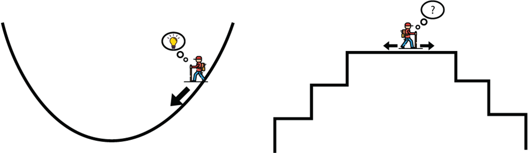
Performing gradient descent to minimize an error function is like descending from a mountain by taking small steps. However, for us to do that, the error function must not be flat (like the one on the right), because in a flat error function, taking a small step will not decrease the error. A good error function is like the one on the left, in which we can easily see the direction we must use to take a step to slightly decrease the error function.

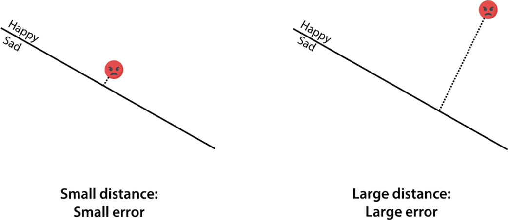
An effective way to measure how bad a classifier misclassifies a point is by measuring the perpendicular distance from the point to the line. For the classifier on the left, this distance is small, whereas for the classifier on the right, the distance is large.

To calculate the total error of a classifier, we add up all the errors, which are the perpendicular distances from the misclassified points. The error is large for the classifier on the left and small for the classifier on the right. Thus, we conclude that the classifier on the right is better.

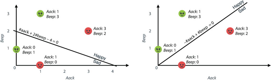
On the left we have classifier 1, and on the right we have classifier 2.

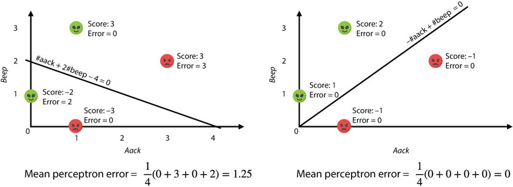
Classifier 1 has an error of 1.25, whereas classifier 2 has an error of 0. Thus, we conclude that classifier 2 is better than classifier 1.

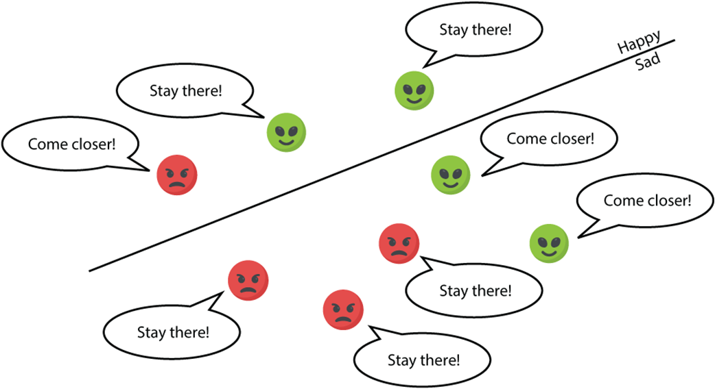
Case 1 (left): A point that is correctly classified tells the line to stay where it is. Case 2 (right): A point that is misclassified tells the line to move closer toward it.

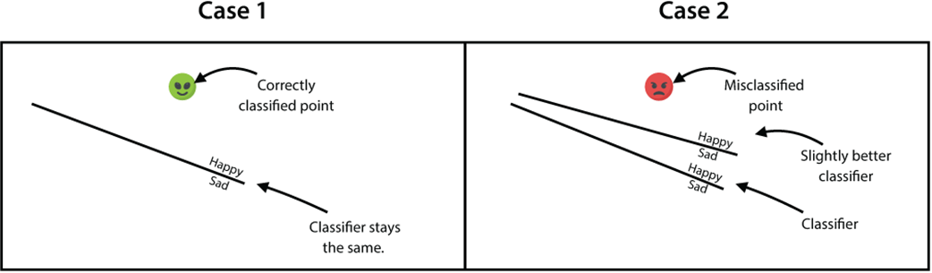
Each point tells the classifier what to do to make life better for itself. The points that are correctly classified tell the line to stay still. The points that are misclassified tell the line to move slightly toward them.

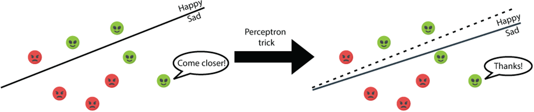
If we apply the perceptron trick to a classifier and a misclassified point, the classifier moves slightly toward the point.

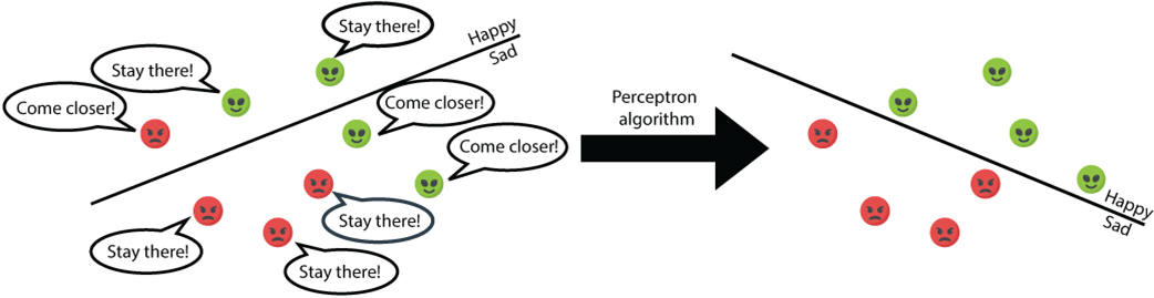
If we apply the perceptron trick many times, each time picking a random point, we can imagine that we’ll obtain a classifier that classifies most points correctly.

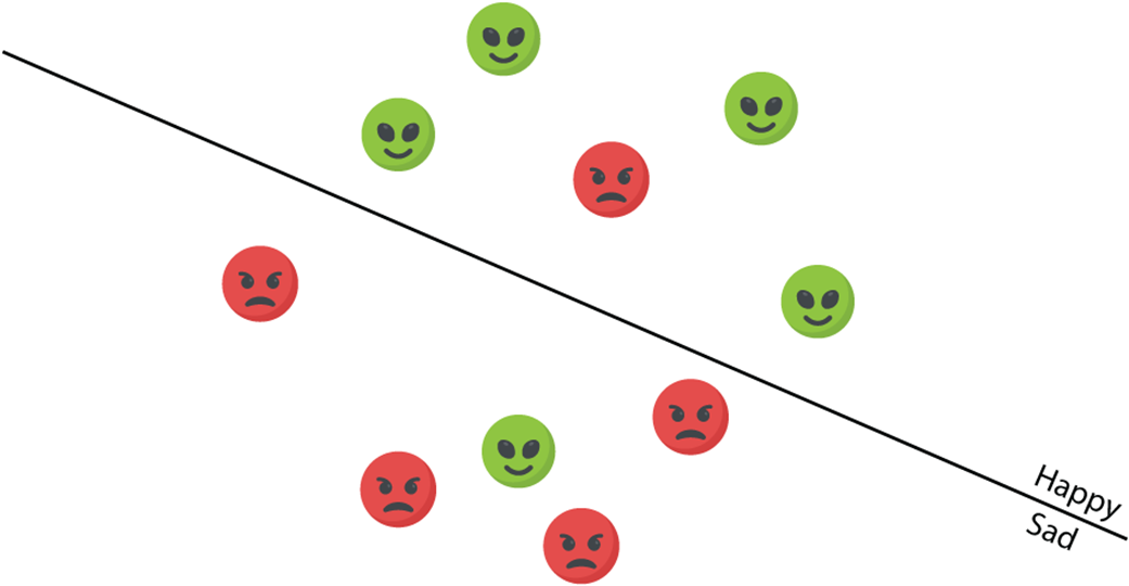
A dataset with two classes that are impossible to separate with a line. The perceptron algorithm is then trained to find a line that separates them as best as possible.

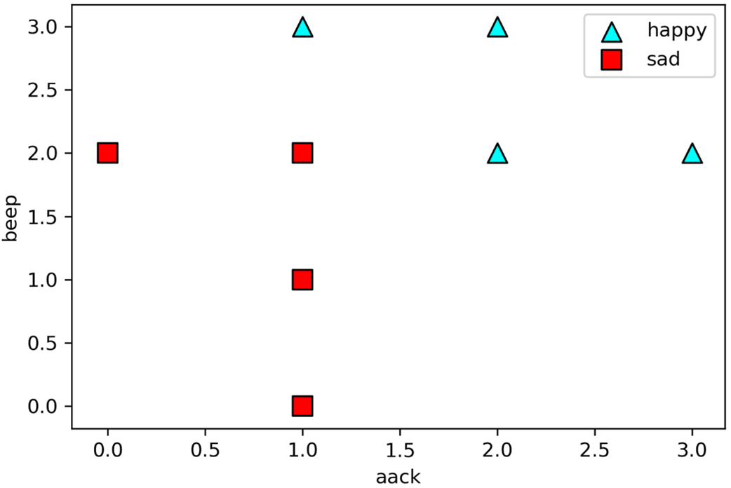
The plot of our dataset. Triangles are happy aliens, and squares are sad aliens.

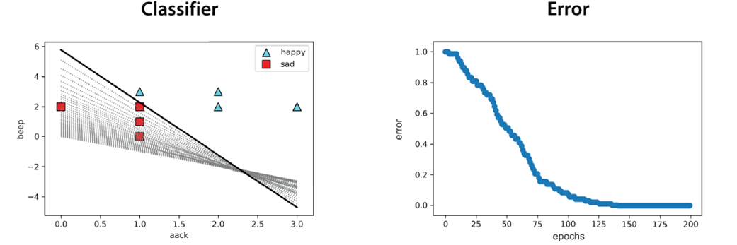
Left: The plot of our resulting classifier. Notice that it classifies each point correctly. Right: The error plot. Notice that the more epochs we run the perceptron algorithm for, the lower the error gets.

FAQ

What is classification, and how is it different from regression?

Classification predicts a category or state (for example, happy/sad, spam/ham), while regression predicts a number. Both use labeled data and features, but classifiers output discrete labels. This chapter focuses on binary classification and introduces the perceptron as a simple linear classifier.

What is a perceptron and how does it make predictions?

A perceptron assigns a weight to each feature and adds a bias. It computes a score s = w·x + b and applies the step function: ŷ = 1 if s ≥ 0, otherwise 0. Geometrically, in two features it’s a line that splits the plane; in higher dimensions, a hyperplane that splits space.

What do the weights and bias represent in a perceptron?

Weights quantify how much each feature pushes the prediction toward 1 or 0 (e.g., “happy” words get positive weights, “sad” words negative). The bias is the score of the “empty” input and shifts the boundary; it’s equivalent to using a threshold T by setting b = −T. A positive bias classifies the origin as positive; a negative bias classifies it as negative.

How is the decision boundary defined and what are the “positive” and “negative” zones?

The decision boundary is the set of points where w·x + b = 0. Points with w·x + b ≥ 0 lie in the positive zone (predicted 1), and those with w·x + b < 0 lie in the negative zone (predicted 0). Flipping the signs of all weights and the bias flips the two zones without changing the boundary.

Can a perceptron handle more than two features?

Yes. With n features, the perceptron still computes ŷ = step(w·x + b). The decision boundary becomes an (n−1)-dimensional hyperplane that splits n‑dimensional space into two regions. In sentiment analysis, each word can be a feature with its own weight.

How do we evaluate how good a perceptron is?

This chapter uses the perceptron error: for correctly classified points, error = 0; for misclassified points, error = |w·x + b|. The mean perceptron error is the average of those errors over the dataset. It’s preferred to simple misclassification counts (too coarse) or exact distances (more complex derivatives) because it’s smooth enough for optimization and reflects mistake severity.

What is the perceptron trick (the core update step)?

For a point (x, y) with prediction ŷ, update the parameters by: w ← w + h(y − ŷ)x and b ← b + h(y − ŷ), where h is the learning rate. If the point is correct, no change. If it’s a false positive (ŷ=1, y=0), the update decreases the score; if it’s a false negative (ŷ=0, y=1), it increases the score.

What are the steps and hyperparameters of the perceptron algorithm?

- Initialize w and b (often randomly). - Repeat for multiple epochs: pick data (one point or a batch), apply the perceptron trick, and monitor the mean perceptron error. - Stop after a fixed number of epochs, when error is below a threshold, or when error plateaus. Key hyperparameters: learning rate (h) and number of epochs; choice of stochastic, mini‑batch, or batch updates.

What happens if the data are not linearly separable?

A single perceptron can’t perfectly separate such data (e.g., XOR). The algorithm will still find a boundary that minimizes mistakes according to the error function, but some points will remain misclassified. More expressive models (e.g., multilayer perceptrons, logistic regression, SVMs) can handle many non‑linear patterns.

How do I implement a perceptron from scratch and with scikit‑learn?

From scratch: implement score (w·x + b), step, prediction, the perceptron error, the perceptron trick, and loop over epochs to update w and b while tracking mean error. With scikit‑learn: create Perceptron(), call fit(X, y), then use predict(X); learned parameters are in coef_ (weights) and intercept_ (bias). Both approaches should yield a separating boundary on linearly separable data.

Our dataset of aliens. We have recorded their mood (happy or sad) and the sentence they keep repeating. Now a fifth alien comes in, saying a different sentence. Do we predict that this alien is happy or sad?

A plot of the dataset of aliens. In the horizontal axis we plot the number of appearances of the word aack, and in the vertical axis, the appearances of the word beep.

The plot of the new dataset of aliens. Notice that the happy ones tend to be above and to the right, and the sad ones below and to the left.

The classifier for the new dataset of aliens. It is again a line that splits the happy and the sad aliens.

This line splits the dataset well. Note that it makes only three mistakes: two on the happy zone and one on the sad zone.

The step function is useful in the study of perceptron models. The output of the step function is 0 when the input is negative and 1 otherwise.

A sentence with three words can be plotted as a point in space. In this case, a sentence with the word aack five times, beep eight times, and crack three times is plotted in the point with coordinates (5,8,3).

A dataset of sentences with three words is plotted in three dimensions. The classifier is represented by a plane that splits the space into two regions.

Left: a bad classifier, which doesn’t really split the points well. Right: a good classifier. Can we think of an error function that assigns a high number to the bad classifier and a low number to the good one?

An effective way to measure how bad a classifier misclassifies a point is by measuring the perpendicular distance from the point to the line. For the classifier on the left, this distance is small, whereas for the classifier on the right, the distance is large.

To calculate the total error of a classifier, we add up all the errors, which are the perpendicular distances from the misclassified points. The error is large for the classifier on the left and small for the classifier on the right. Thus, we conclude that the classifier on the right is better.

On the left we have classifier 1, and on the right we have classifier 2.

Classifier 1 has an error of 1.25, whereas classifier 2 has an error of 0. Thus, we conclude that classifier 2 is better than classifier 1.

Case 1 (left): A point that is correctly classified tells the line to stay where it is. Case 2 (right): A point that is misclassified tells the line to move closer toward it.

Each point tells the classifier what to do to make life better for itself. The points that are correctly classified tell the line to stay still. The points that are misclassified tell the line to move slightly toward them.

If we apply the perceptron trick to a classifier and a misclassified point, the classifier moves slightly toward the point.

If we apply the perceptron trick many times, each time picking a random point, we can imagine that we’ll obtain a classifier that classifies most points correctly.

A dataset with two classes that are impossible to separate with a line. The perceptron algorithm is then trained to find a line that separates them as best as possible.

The plot of our dataset. Triangles are happy aliens, and squares are sad aliens.

Left: The plot of our resulting classifier. Notice that it classifies each point correctly. Right: The error plot. Notice that the more epochs we run the perceptron algorithm for, the lower the error gets.

pro $24.99 per month

lite $19.99 per month

team

pro

team

pro

team