3 Drawing a line close to our points: Linear regression
This chapter builds an intuitive, visual understanding of linear regression as the task of drawing a straight line that stays as close as possible to a cloud of data points in order to predict continuous quantities (like house prices). It reframes the usual algebra and calculus in terms of points, lines, slope, and intercept, and introduces core machine learning ideas—features, labels, weights, bias, correlation, and the remember–formulate–predict workflow. Starting from a single-feature example (rooms vs. price) and extending to multiple features, it shows how the slope encodes how much the prediction changes per unit of a feature and the intercept captures a baseline value, while noting how positive and negative weights reflect positive and negative correlations.
To find the best-fitting line, the chapter develops a step‑by‑step training procedure: begin with a random line and nudge it closer to the data repeatedly. It first presents a simple geometric “move-toward-the-point” trick, then improves it with the absolute and square tricks, which use the learning rate and signed errors to update slope and intercept more reliably. It formalizes error functions—absolute error, square error, and their mean and root-mean-square variants—to quantify model quality, explains gradient descent as a way to minimize these errors, and discusses practical training choices like when to stop (by monitoring error curves) and whether to update with single points, batches, or mini-batches. Along the way, it sketches clean pseudocode and compact Python implementations to show the ideas in action.
Bridging to real data, the chapter demonstrates building a housing price model with scikit‑learn, highlighting crucial preprocessing steps (handling missing values, scaling numerics, and one‑hot encoding categoricals), inspecting learned coefficients, and making predictions. When data relationships are nonlinear, it introduces polynomial regression—augmenting features with powers of the inputs—to fit curves instead of lines, and flags the importance of choosing model complexity wisely to avoid underfitting or overfitting. It closes by distinguishing parameters (learned weights and bias) from hyperparameters (learning rate, epochs, polynomial degree, and more), and surveys practical applications where regression shines—from recommendation systems that predict watch time or spend to healthcare tasks like estimating life expectancy or length of stay.

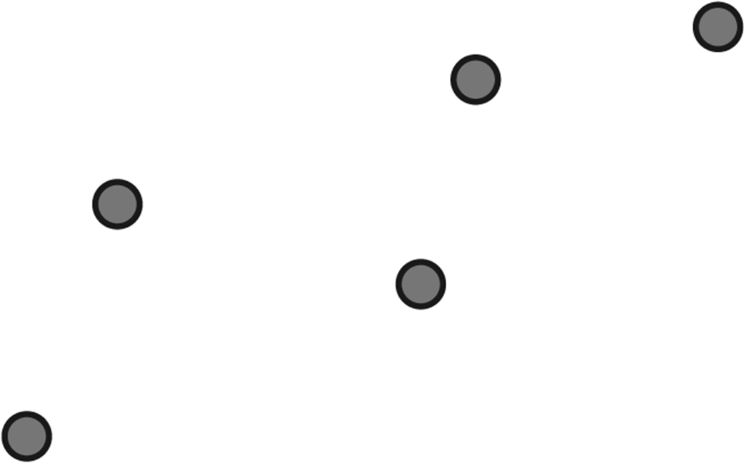
Some points that roughly look like they are forming a line
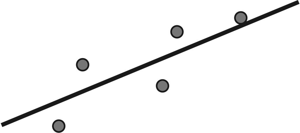
A line that passes close to the points
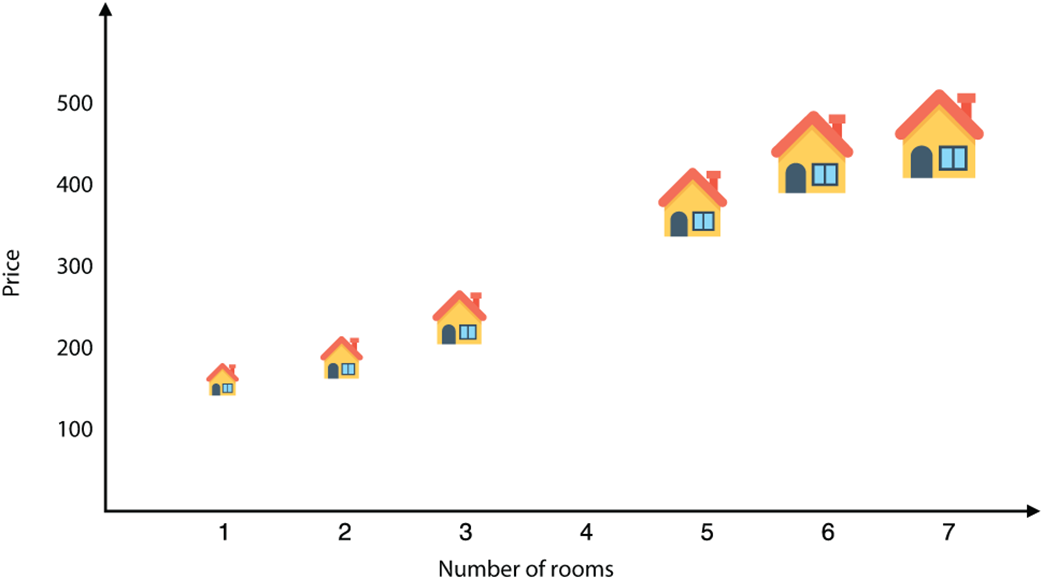
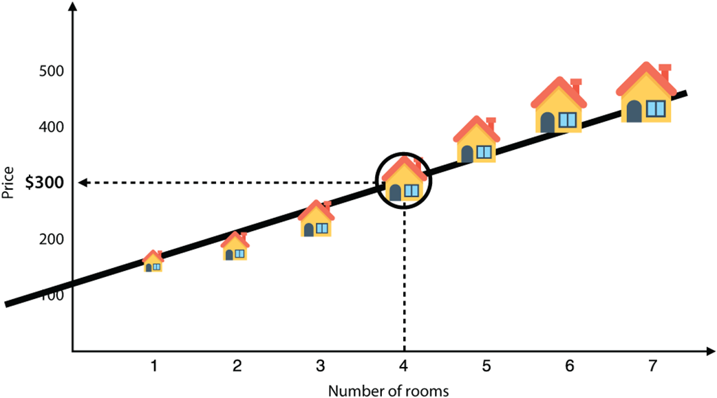
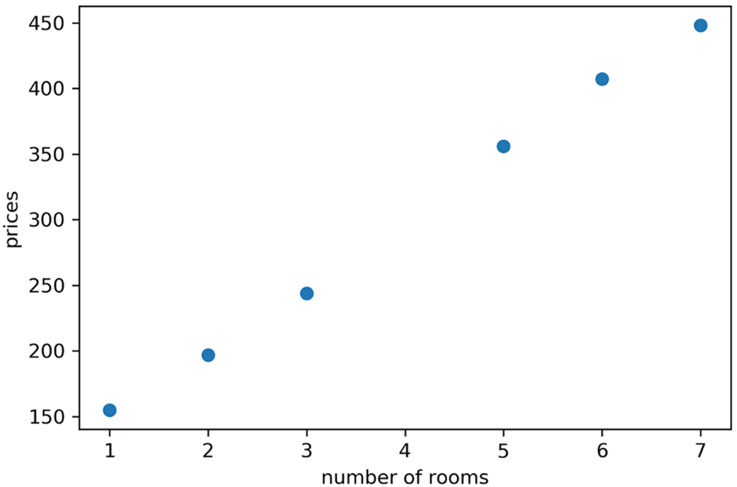
Plot of the dataset in table 3.2. The horizontal axis represents the number of rooms, and the vertical axis represents the price of the house.
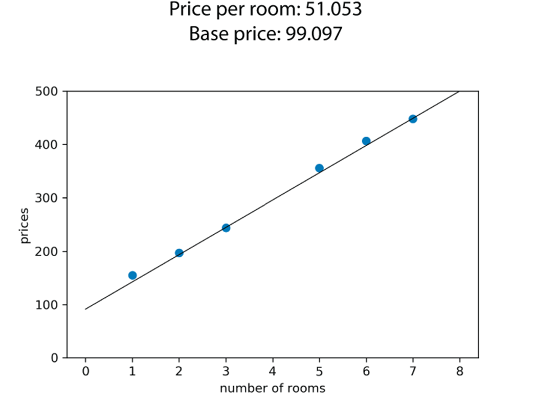
The model we formulate is the line that goes as close as possible to all the houses.
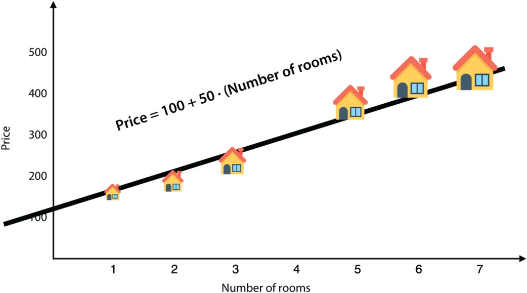
Our task is now to predict the price of the house with four rooms. Using the model (line), we deduce that the predicted price of this house is $300.
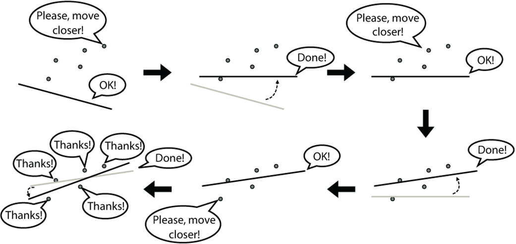
An illustration of the linear regression algorithm. We start at the top left with a random line and end in the bottom left with a line that fits the dataset well. At each stage, two things happen: (1) we pick a random point, and (2) the point asks the line to move closer to it. After many iterations, the line will be in a good position. This figure has only three iterations for illustrative purposes, but in real life, many more iterations are needed.
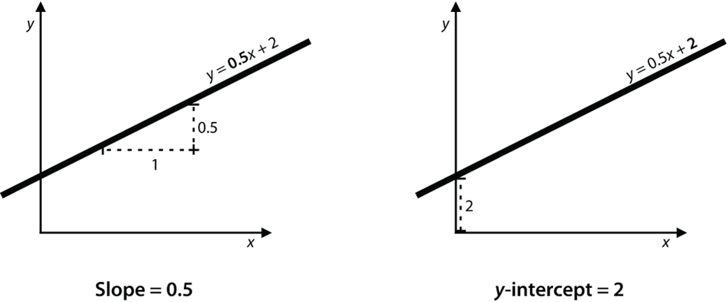
The line with equation y = 0.5x + 2 has slope 0.5 (left) and y-intercept 2 (right).
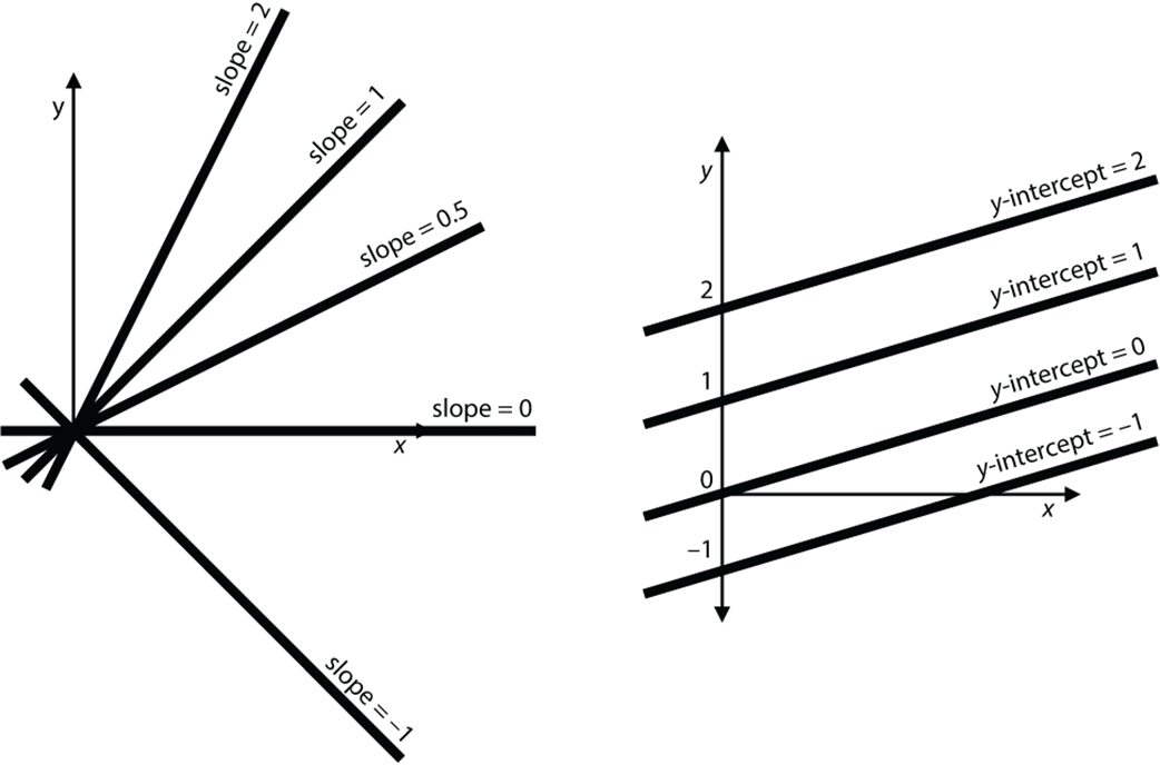
Some examples of slope and y-intercept. On the left, we see several lines with the same intercept and different slopes. Notice that the higher the slope, the steeper the line. On the right, we see several lines with the same slope and different y-intercepts. Notice that the higher the y-intercept, the higher the line is located.
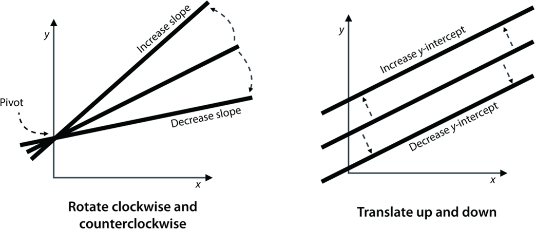
Left: Increasing the slope rotates the line counterclockwise, whereas decreasing the slope rotates it clockwise. Right: Increasing the y-intercept translates the line upward, whereas decreasing the y-intercept translates it downward.
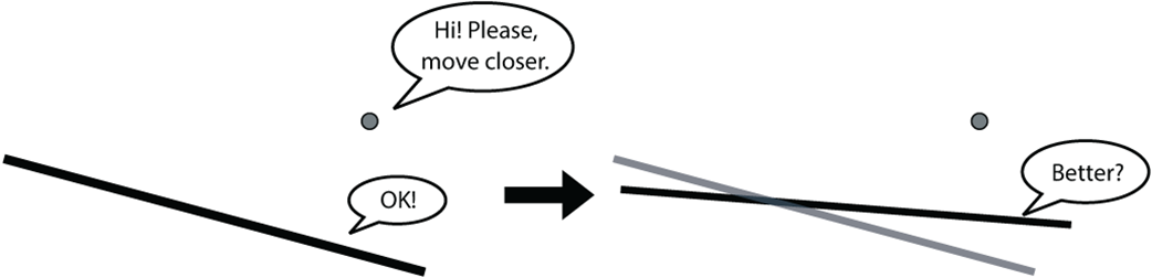
Our goal is to rotate and translate the line by a small amount to get closer to the point.
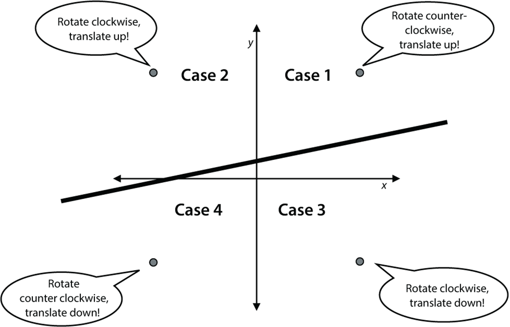
The four cases. In each of these we must rotate the line and translate it in a different way to move the line closer to the corresponding point.
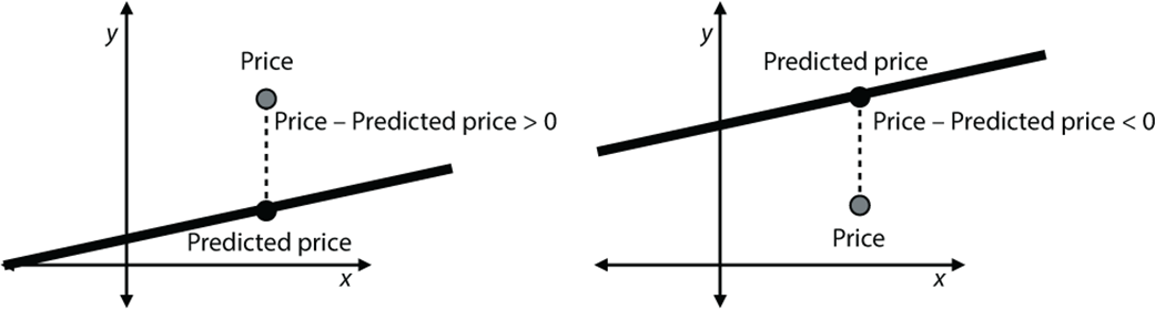
Left: When the point is above the line, the price is larger than the predicted price, so the difference is positive. Right: When the point is below the line, the price is smaller than the predicted price, so the difference is negative.
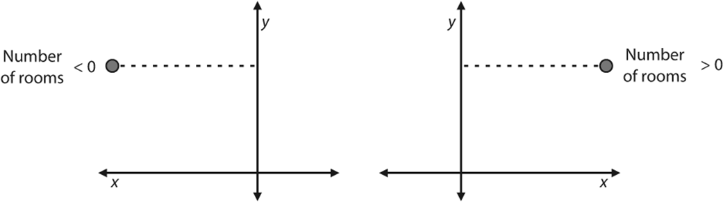
Left: When the point is to the left of the y-axis, the number of rooms is negative. Right: When the point is to the right of the y-axis, the number of rooms is positive.
The plot of the points in table 3.2
The plot of the points in table 3.2 and the line that we obtained with the linear regression algorithm
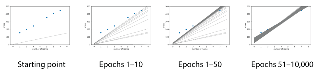
Drawing some of the lines in our algorithm, as we approach a better solution. The first graphic shows the starting point. The second graphic shows the first 10 epochs of the linear regression algorithm. Notice how the line is moving closer to fitting the points. The third graphic shows the first 50 epochs. The fourth graphic shows epochs 51 to 10,000 (the last epoch).
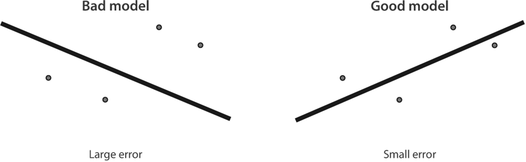
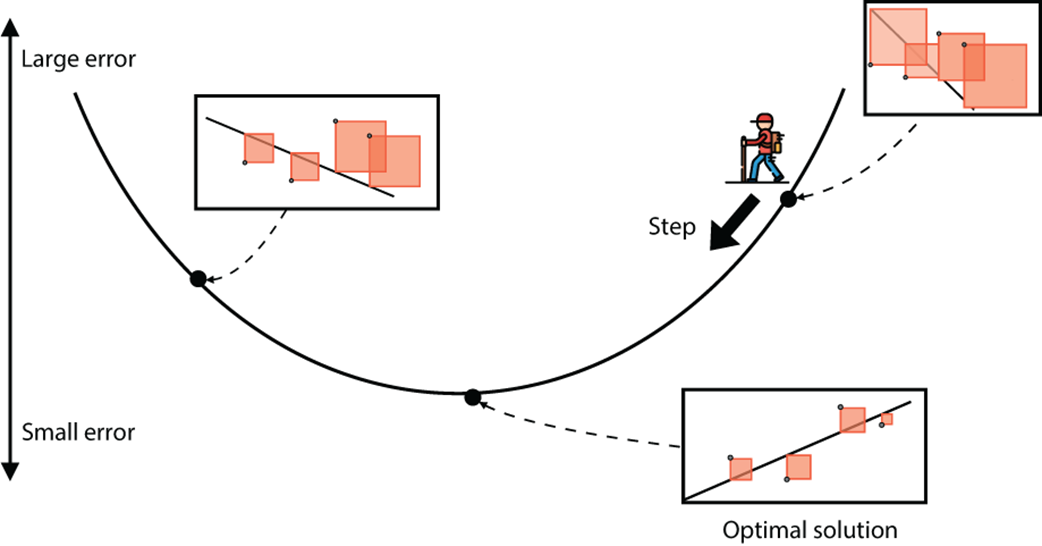
Two models, a bad one (on the left) and a good one (on the right). The bad one is assigned a large error, and the good one is assigned a small error.
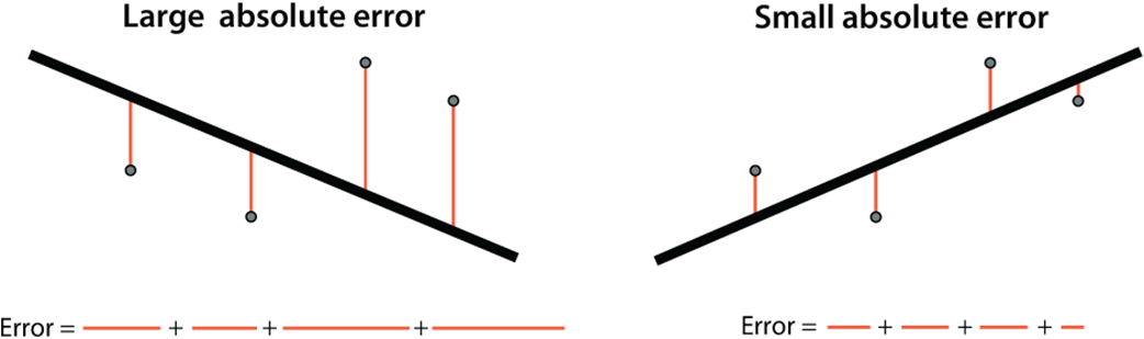
The absolute error is the sum of the vertical distances from the points to the line. Note that the absolute error is large for the bad model on the left and small for the good model on the right.
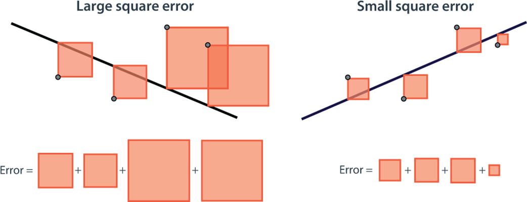
The square error is the sum of the squares of the vertical distances from the points to the line. Note that the square error is large for the bad model on the left and small for the good model on the right.
We are on top of Mount Errorest and wish to get to the bottom, but we can’t see very far. A way to go down is to look at all the directions in which we can take one step and figure out which one helps us descend the most. Then we are one step closer to the bottom.
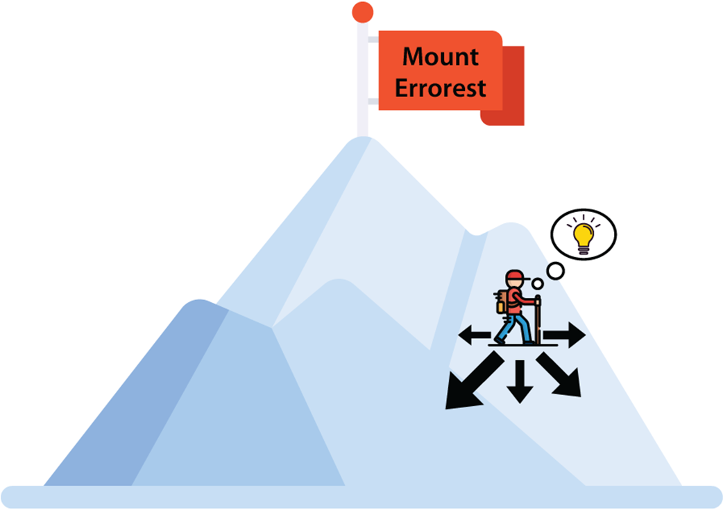
The way to descend from the mountain is to take that one small step in the direction that makes us descend the most and to continue doing this for a long time.
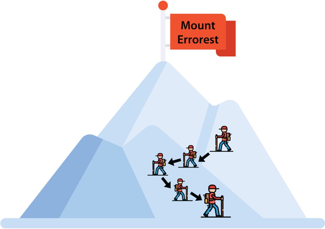
Each point on this mountain corresponds to a different model. The points below are good models with a small error, and the points above are bad models with a large error. The goal is to descend from this mountain. The way to descend is by starting somewhere and continuously taking a step that makes us descend. The gradient will help us decide in what direction to take a step that helps us descend the most.
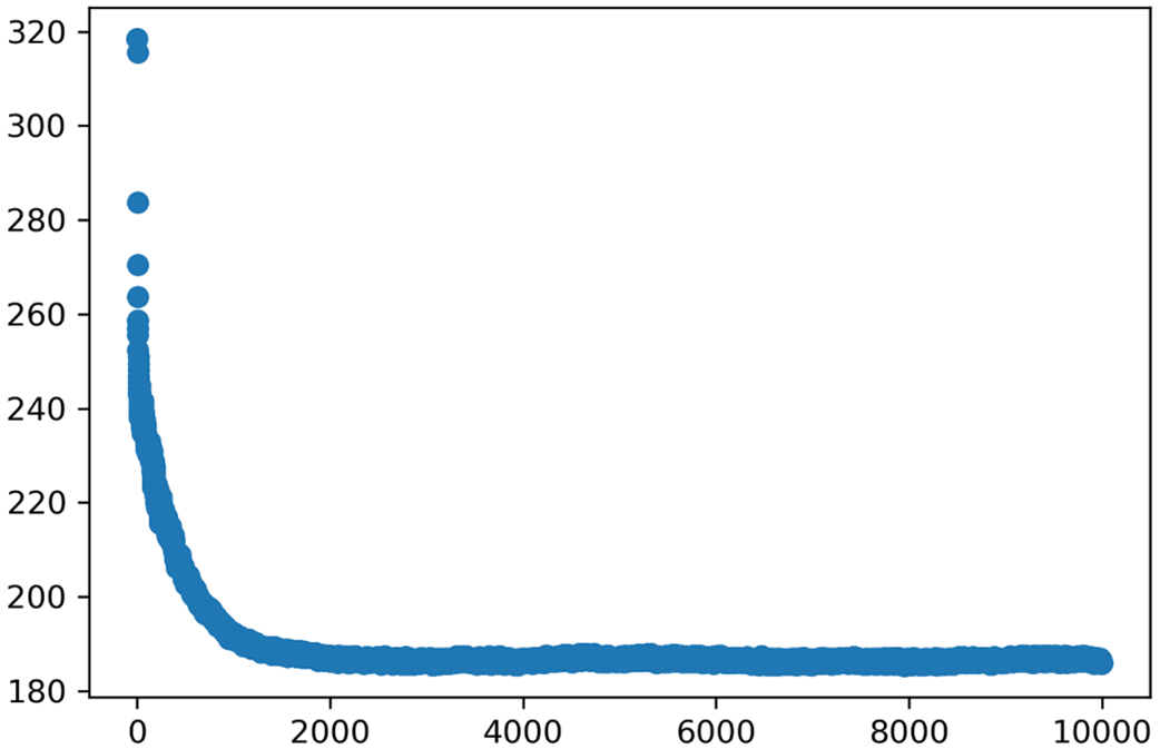
The plot of the root mean square error for our running example. Notice how the algorithm succeeded in reducing this error after a little over 1,000 iterations. This means that we don’t need to keep running this algorithm for 10,000 iterations, because around 2,000 of them do the job.
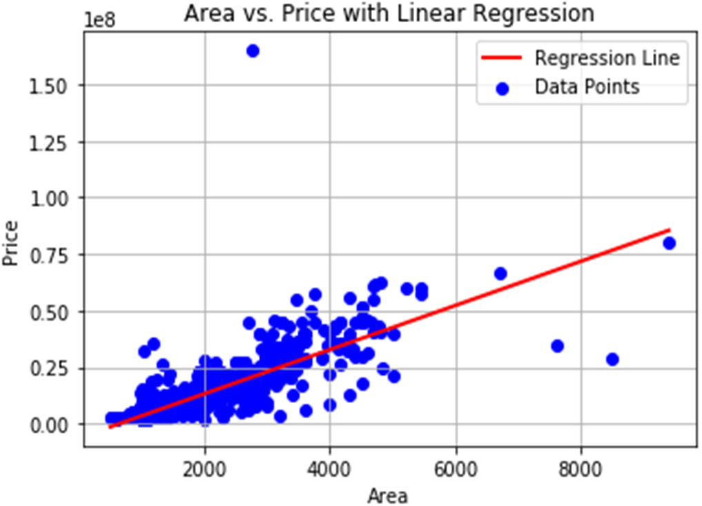
The Hyderabad housing prices dataset restricted to area and price. The line is the model we’ve obtained using only the area feature to predict the price.
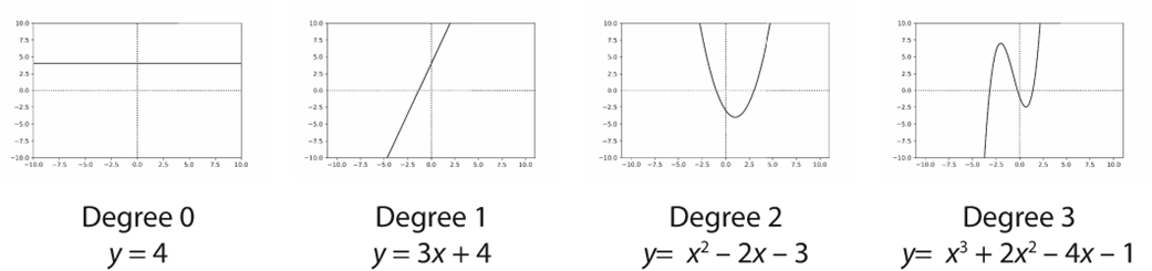
Polynomials are functions that help us model our data better. Here are the plots of four polynomials of degrees 0 to 3. Note that the polynomial of degree 0 is a horizontal line, the polynomial of degree 1 is any line, the polynomial of degree 2 is a parabola, and the polynomial of degree 3 is a curve that oscillates twice.
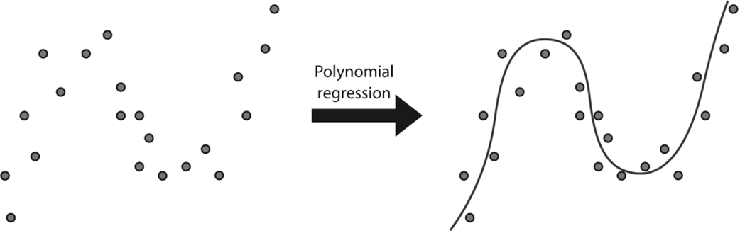
Polynomial regression is useful when it comes to modeling nonlinear data. If our data looks like the left part of the figure, it will be hard to find a line that fits it well. However, a curve will fit the data well, as you can see in the right part of the figure. Polynomial regression helps us find this curve.
FAQ
What is linear regression and what kind of problems does it solve?
Linear regression learns a simple formula that maps features (inputs) to a numeric label (output). Geometrically, with one feature it finds the line y = mx + b that passes as close as possible to the data points. It’s used to estimate quantities such as house prices, watch time, life expectancy, and sales.What do weight (slope) and bias (y-intercept) mean in a linear model?
The weight (slope, m) tells how much the prediction changes when the feature increases by one unit (for housing, the price change per extra room). The bias (y-intercept, b) is the baseline prediction when all features are zero (the base price).How do we train a linear regression model from data?
Start with random m and b, repeatedly pick a data point, compute the model’s error on it, and nudge m and b to reduce that error. After many small updates (epochs), the line settles near the points, yielding a good fit and usable predictions.What are the “simple,” “absolute,” and “square” tricks for updating the line?
- Simple trick: adjust slope and intercept up or down depending on whether a point lies above or below the line and on its position, using small handpicked steps.- Absolute trick: use the sign of (price − prediction) and the feature value to update in two cases, with a fixed small step size.
- Square trick: update both slope and intercept by amounts proportional to r × (price − prediction) and (price − prediction), respectively, each scaled by a small learning rate. It unifies cases and usually works best.

 Grokking Machine Learning, Second Edition ebook for free
