Overview

10 Combining building blocks to gain more power: Neural networks

Neural networks are introduced as powerful, flexible models built by combining simple building blocks (perceptrons) into layered structures that can learn complex, nonlinear decision boundaries. Beginning from an intuitive two-line sentiment example, the chapter shows how stacking linear classifiers and passing their outputs forward creates richer boundaries than any single line can provide. This brain-inspired view—inputs weighted and summed, passed through activation functions, and organized into input, hidden, and output layers—explains why neural networks excel across tasks like vision, language, and other real-world problems, for both classification and regression.

The chapter details the mechanics and architecture of fully connected networks: nodes, weights, biases, activations, and depth, and how boundaries grow more expressive with each hidden layer. Training is framed around defining a suitable error function (log loss for classification) and optimizing parameters via gradient descent using backpropagation. Practical challenges are addressed: vanishing gradients (mitigated by activation choices like ReLU over sigmoid/tanh), overfitting (handled with regularization and dropout), and the need to tune hyperparameters such as learning rate, epochs, batch size, architecture, and regularization strength. Multi-class outputs are handled with softmax, and simple adjustments (removing the final squashing function and switching to regression losses) turn the same machinery into regression models.

Hands-on sections demonstrate Keras implementations on a 2D nonlinear dataset and MNIST digit recognition, highlighting how little code is needed to define architectures, compile with modern optimizers, and train effectively—while also encouraging validation and hyperparameter exploration. The chapter broadens to specialized architectures and practices: convolutional neural networks for images (often with transfer learning), recurrent variants such as RNNs, LSTMs, and GRUs for sequence and language tasks, and generative adversarial networks for realistic content generation. Throughout, the emphasis is on building intuition for how layered perceptrons compose into powerful models, how to train them robustly, and how to adapt them to different problem types.

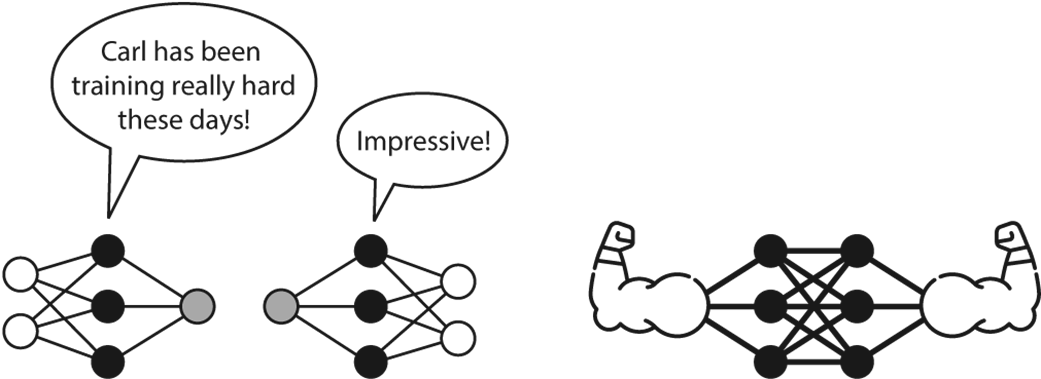
A neural network. It may look complicated, but in the next few pages, we will demystify this image.

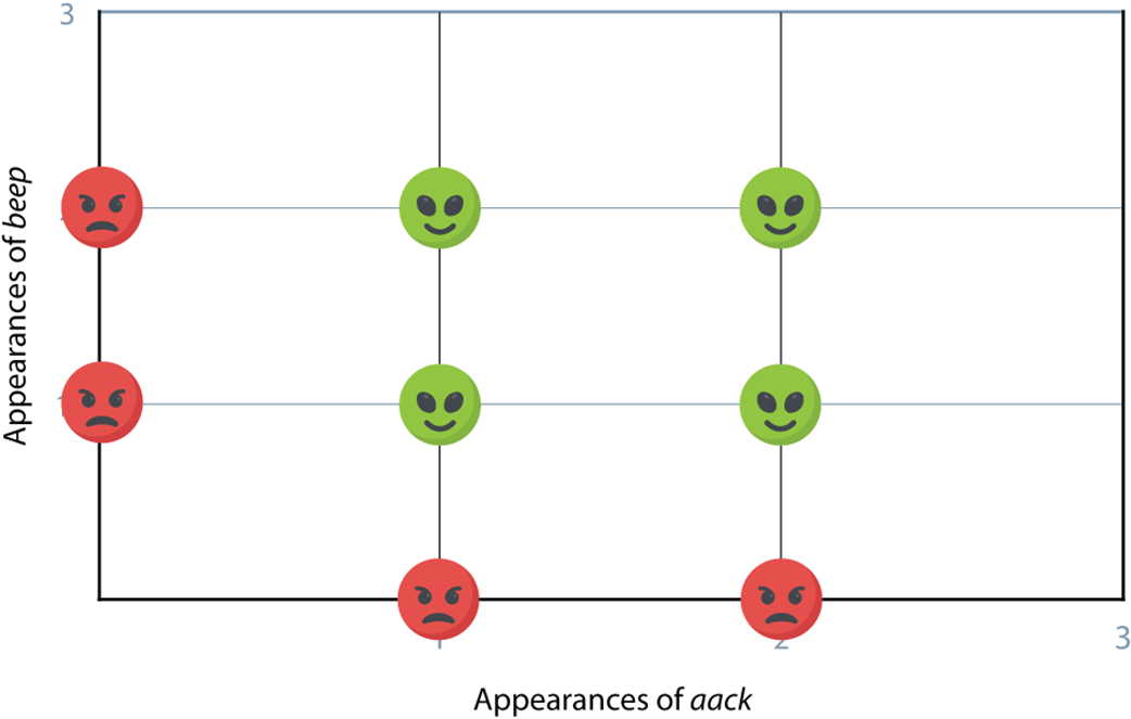
The plot of the dataset in table 10.1. The horizontal axis corresponds to the number of appearances of the word aack, and the vertical axis to the number of appearances of the word beep. The happy faces correspond to the happy aliens, and the sad faces to the sad aliens.

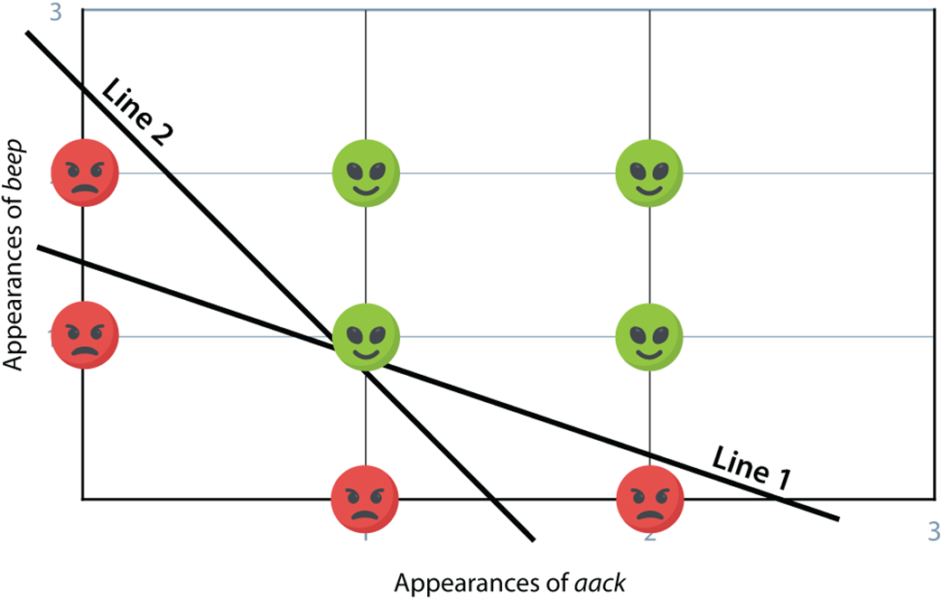
The happy and the sad points in our dataset cannot be divided by one line. However, drawing two lines separates them well—the points above both lines can be classified as happy, and the remaining points as sad. Combining linear classifiers this way is the basis for neural networks.

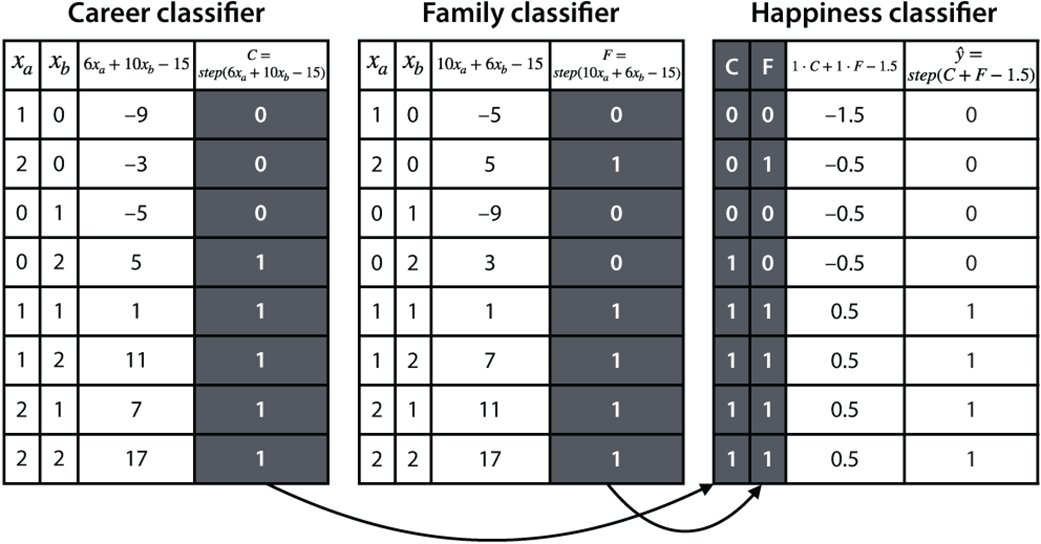
The happiness classifier is formed by the career happiness classifier, the family happiness classifier, and an AND operator. If both the career and family happiness classifiers output a Yes, then so does the happiness classifier. If any of them outputs a No, then the happiness classifier also outputs a No.

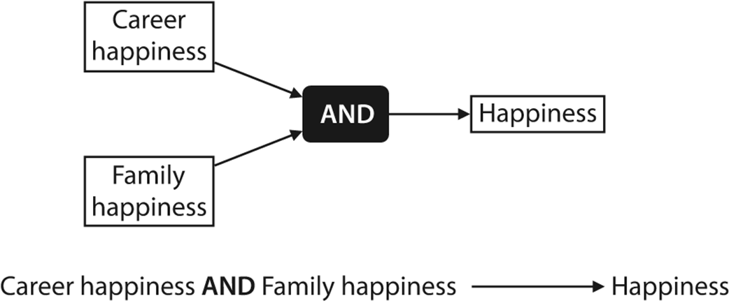
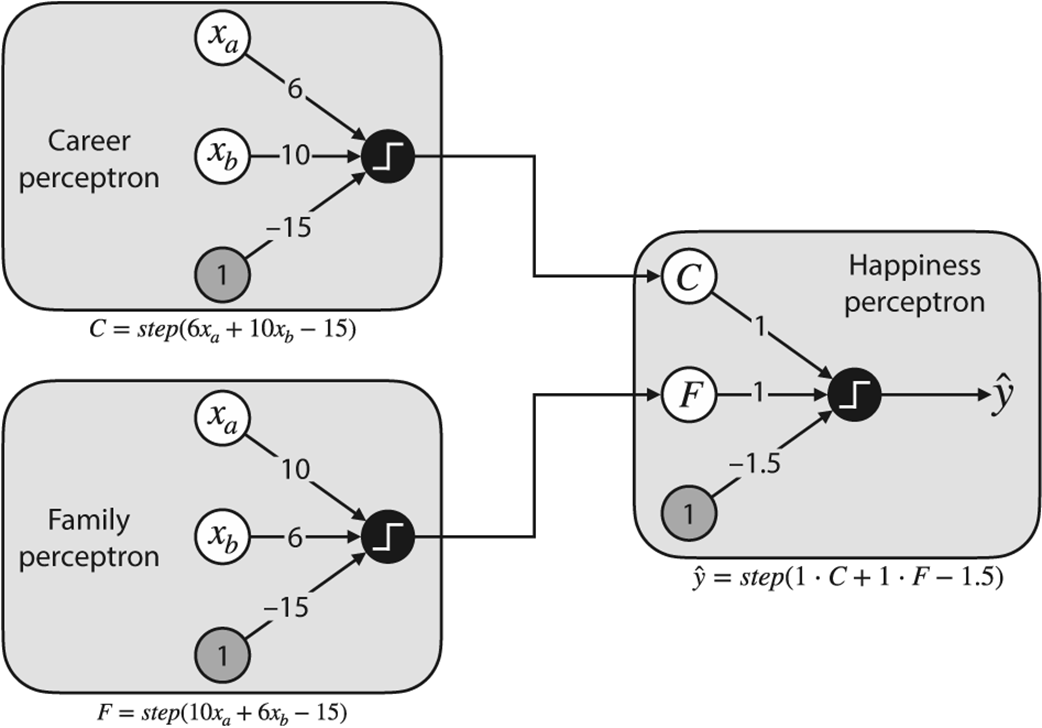
Three perceptron classifiers, one for career happiness, one for family happiness, and one for happiness, which combines the two previous ones. The outputs of the career and family perceptrons are inputs into the happiness perceptron.

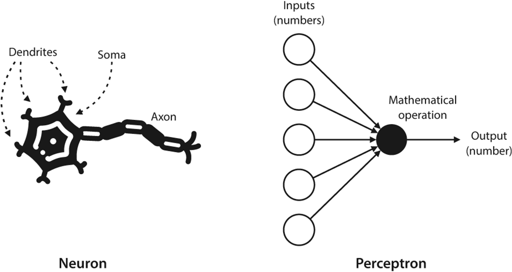
A perceptron is loosely based on a neuron. Left: A neuron with its main components: the dendrites, the soma, and the axon. Signals come in through the dendrites, get processed in the soma, and get sent to other neurons through the axon. Right: A perceptron. The nodes in the left correspond to numerical inputs, the node in the middle performs a mathematical operation and outputs a number.

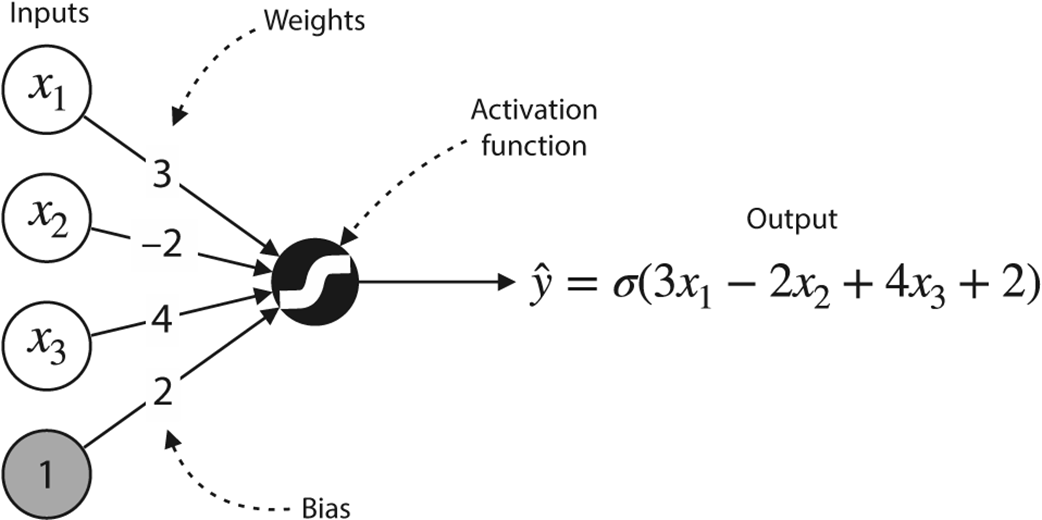
A visual representation of a perceptron. The inputs (features and bias) appear as nodes on the left, and the weights and bias are on the edges connecting the input nodes to the main node in the middle. The node in the middle takes the linear combination of the weights and the inputs, adds the bias, and applies the activation function, which in this case is the sigmoid function. The output is the prediction given by the formula ŷ = σ(3x1 – 2x2 + 4x3 + 2).

Neural networks are meant to (loosely) emulate the structure of the brain. Left: The neurons are connected inside the brain in a way that the output of a neuron becomes the input to another neuron. Right: The perceptrons are connected in a way that the output of a perceptron becomes the input to another perceptron.

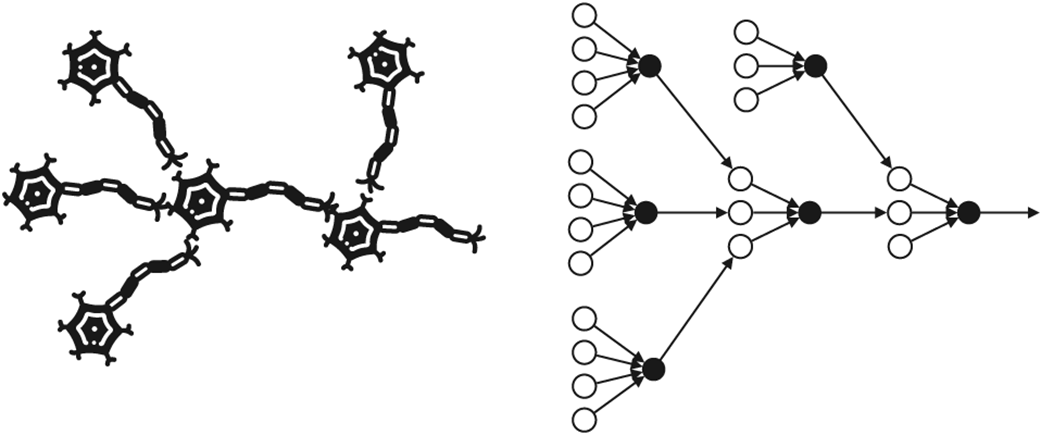
When we connect the outputs of the career and family perceptrons into the happiness perceptron, we get a neural network. This neural network uses the step function as an activation function.

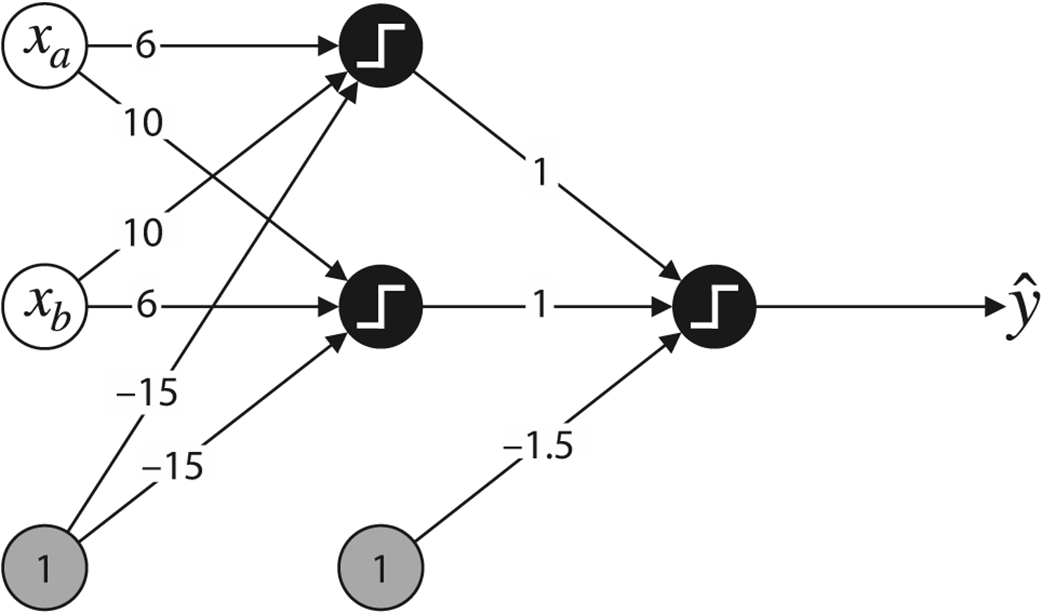
A cleaned-up version of the diagram in figure 10.9. In this diagram, the features xa and xb, and the bias are not repeated. Instead, each of them connects to both of the nodes at the right, nicely combining the three perceptrons into the same diagram.

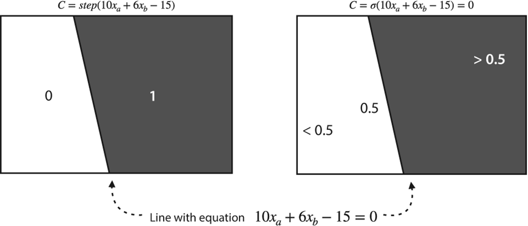
The boundary of a perceptron is a line. Left: For a discrete perceptron, the points on one side of the line are given a prediction of 0, and the points on the other side a prediction of 1. Right: For a continuous perceptron, the points are all given a prediction in the interval (0,1). In this example, the points at the very left get predictions close to 0, those at the very right get predictions close to 1, and those over the line get predictions of 0.5.

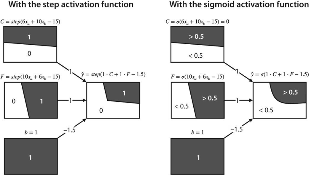
To build a neural network, we use the outputs of two perceptrons and a bias node (represented by a classifier that always outputs a value of 1) to a third perceptron. The boundary of the resulting classifier is a combination of the boundaries of the input classifiers. On the left, we see the boundary obtained using the step function, which is a broken line. On the right, we see the boundary obtained using the sigmoid function, which is a curve.

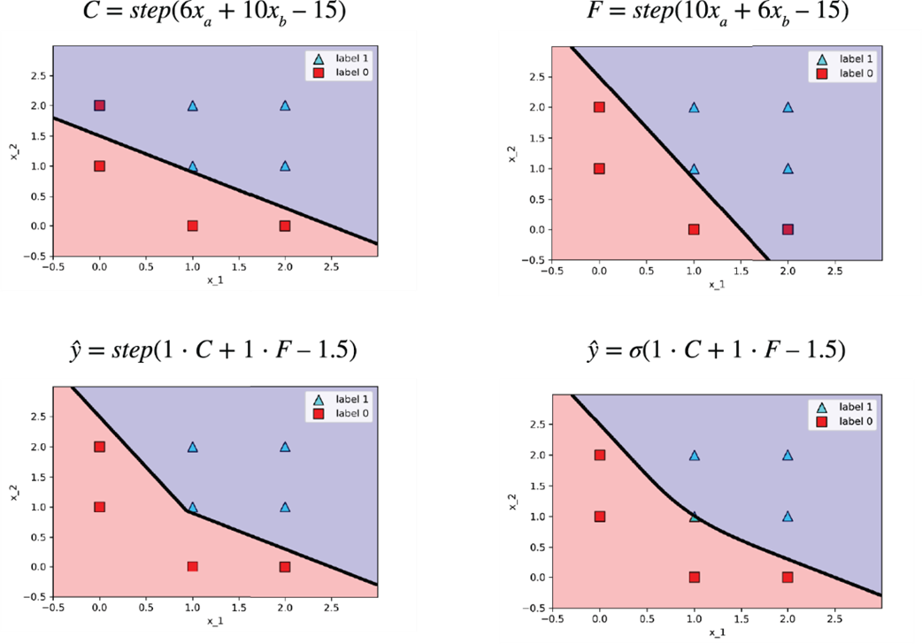
The plots of the boundaries of the classifiers. Top: The two linear classifiers, the career (left) and family (right) classifiers. Bottom: The two neural networks, using the step function (left) and the sigmoid function (right).

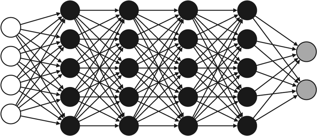
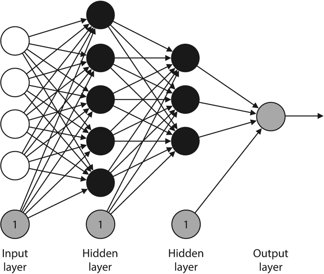
The general architecture of a neural network. The nodes are divided into layers, where the leftmost layer is the input layer, the rightmost layer is the output layer, and all the layers in between are hidden layers. All the nodes in a layer are connected to all the (non-bias) nodes in the next layer.

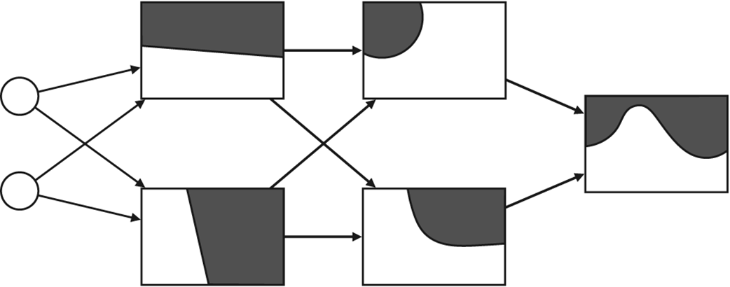
The way I like to visualize neural networks. Each of the nodes corresponds to a classifier, and this classifier has a well-defined boundary. The nodes in the first hidden layer all correspond to linear classifiers (perceptrons), so they are drawn as lines. The boundaries of the nodes in each layer are formed by combining the boundaries from the previous layer. Therefore, the boundaries get more and more complex in each hidden layer. In this diagram, we have removed the bias nodes.

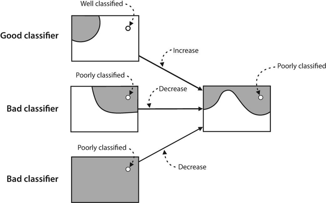
A mental picture of backpropagation. At each step of the training process, the weights of the edges are updated. If a classifier is good, its weight gets increased by a small amount, and if it is bad, its weight gets decreased.

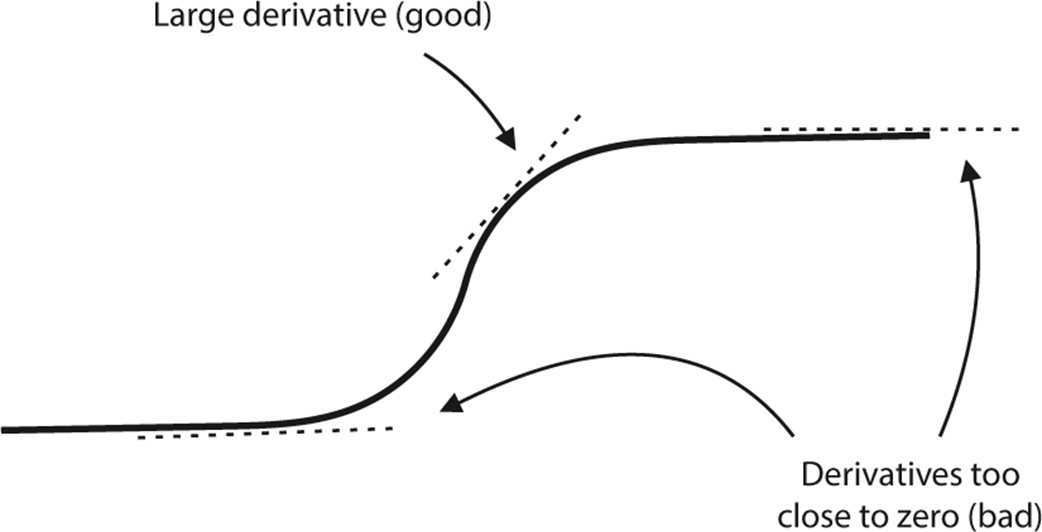
The sigmoid function is flat at the ends, which means that for large positive and negative values, its derivative is very small, hampering the training.

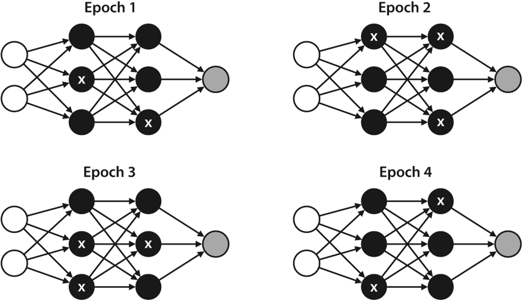
The dropout process. At different epochs, we pick random nodes to remove from the training to give all the nodes an opportunity to update their weights and not have a few single nodes dominating the training.

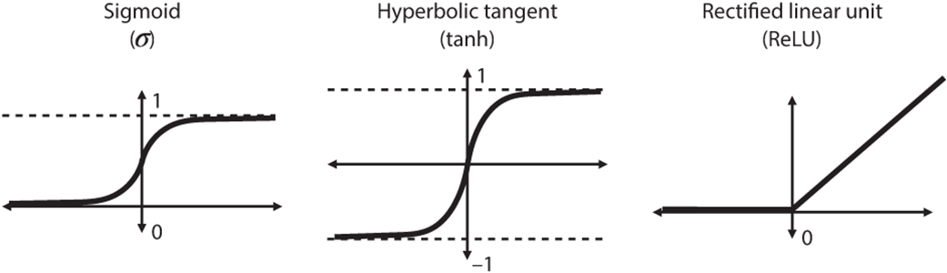
Three different activation functions used in neural networks. Left: The sigmoid function, represented by the Greek letter sigma. Middle: The hyperbolic tangent, or tanh. Right: The rectified linear unit, or ReLU.

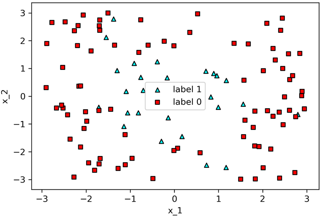
Neural networks are great for nonlinearly separable sets. To test this, we’ll train a neural network on this circular dataset.

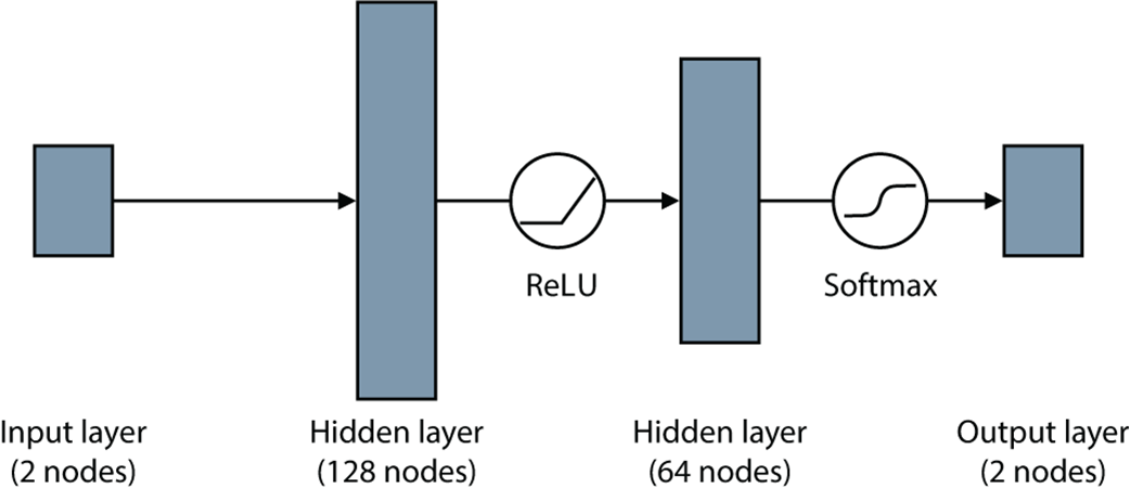
The architecture that we will use to classify our dataset. It contains two hidden layers: one of 128 and one of 64 nodes. The activation function between them is a ReLU, and the final activation function is a softmax.

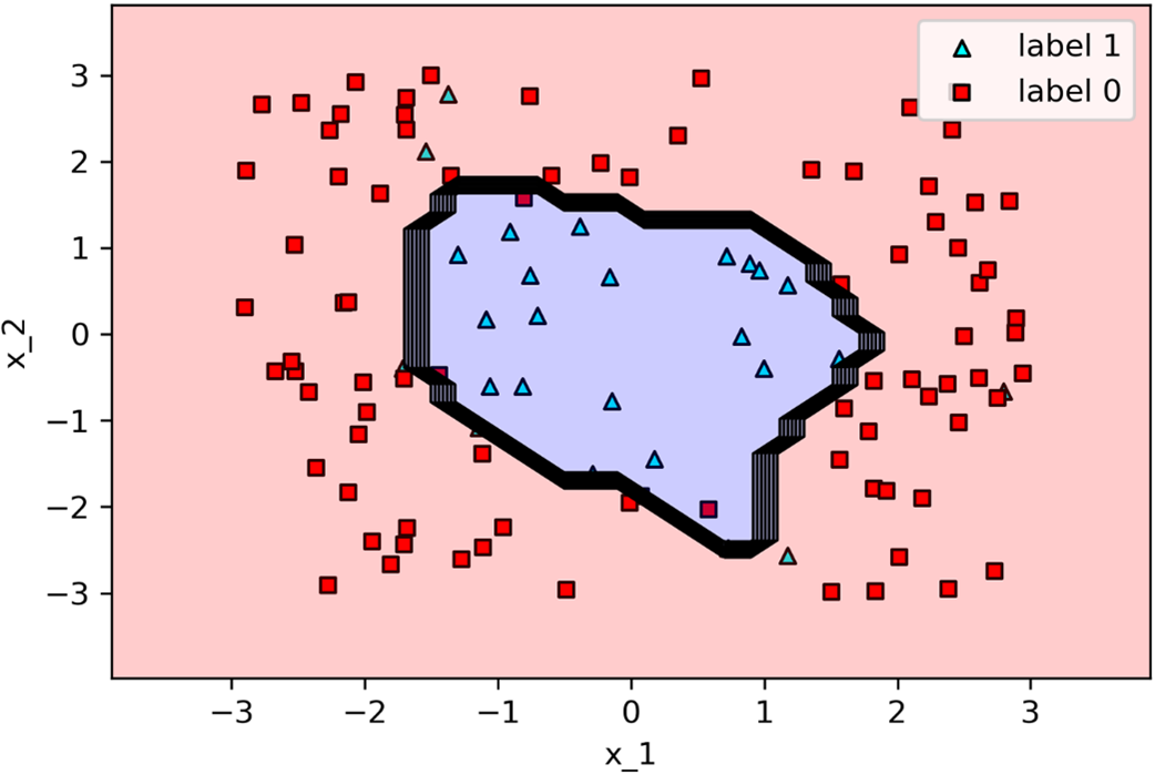
The boundary of the neural network classifier we trained. Notice that it correctly classifies most of the points, with a few exceptions.

Some examples of handwritten digits in MNIST with their labels

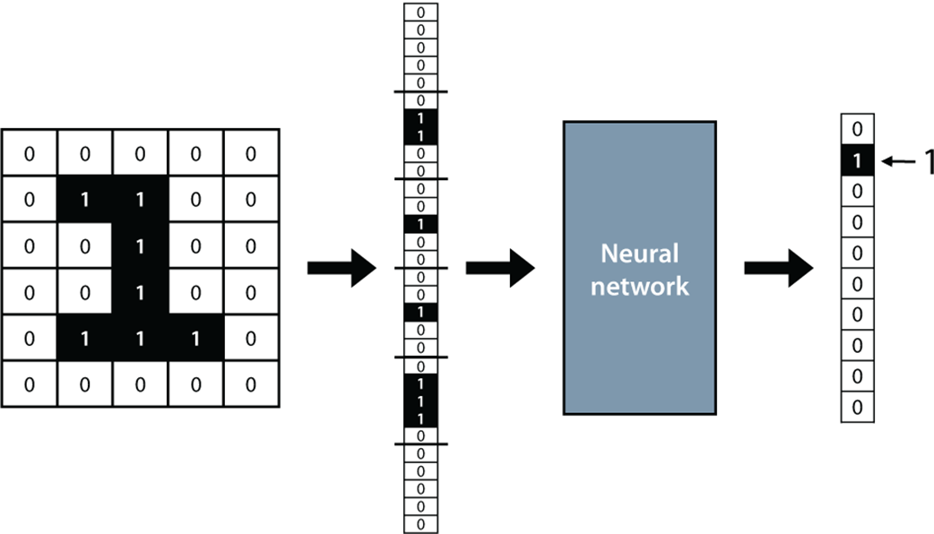
Before training the neural network, we preprocess the images and the labels in the following way. We shape the rectangular image into a long vector by concatenating the rows. We then convert each label into a vector of length 10 with only one non-zero entry in the position of the corresponding label.

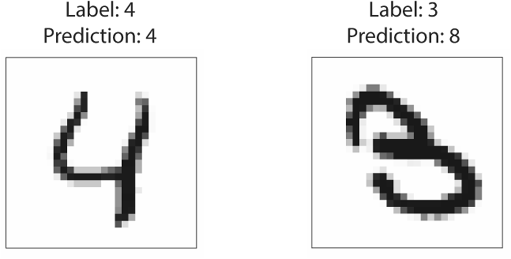
Left: An image of a 4 that has been correctly classified by the neural network. Right: An image of a 3 that has been incorrectly classified as an 8.

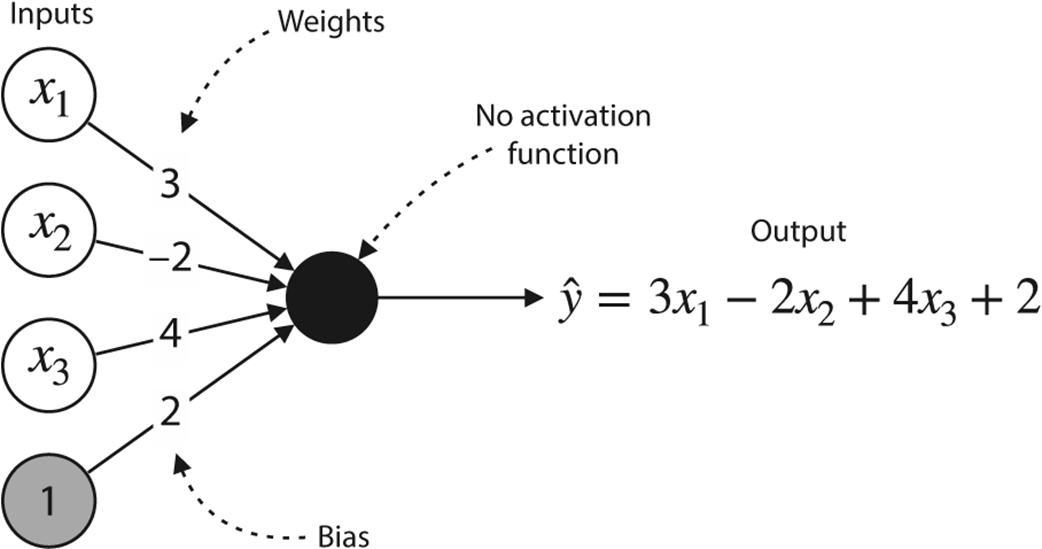
If we remove the activation function from a perceptron, we turn a classification model into a linear regression model. The linear regression model predicts any numerical value, not just one between 0 and 1.

FAQ

What is a neural network and how does it build nonlinear decision boundaries?

A neural network (multilayer perceptron) is a composition of perceptrons arranged in layers. By combining simple linear classifiers (perceptrons) and then feeding their outputs into further perceptrons (e.g., joining two lines with an AND), the network creates nonlinear decision boundaries that can separate data a single line cannot.

How is a neural network structured (nodes, layers, depth, fully connected)?

Inputs feed into hidden layers and then an output layer. The number of non-input layers defines the depth. In a fully connected architecture, every node in one layer connects to every non-bias node in the next layer. Bias nodes exist but are not counted in layer size.

How does a single perceptron (neuron) compute its output?

It multiplies each input by a weight, sums them, adds a bias, and applies an activation function to produce the output: ŷ = f(w·x + b). Using different activations turns this into discrete or continuous outputs.

Which activation functions should I use and why?

- Sigmoid: squashes to (0,1); common in the final layer for binary classification. - Tanh: (-1,1); often better than sigmoid but can still suffer vanishing gradients. - ReLU: max(0,x); mitigates vanishing gradients and is widely used in hidden layers. - Softmax: turns scores into a probability distribution over multiple classes in the output layer.

What do decision boundaries of neural networks look like?

A single perceptron yields a linear boundary (a line/plane). Stacking perceptrons in layers combines boundaries from earlier layers, producing piecewise linear (with step/ReLU) or smoothly curved (with sigmoid/tanh) nonlinear boundaries that can fit complex patterns.

How are neural networks trained with backpropagation?

Initialize weights randomly. Use a loss function (log loss/cross-entropy for classification) to measure error. Backpropagation computes gradients of the loss with respect to all weights and biases and updates them via gradient descent (often with optimizers like Adam) over many epochs.

What common training problems occur and how do we address them?

- Overfitting: use regularization (L1/L2), dropout, and proper validation. - Vanishing gradients: prefer ReLU (or variants) in hidden layers and careful initialization; avoid step functions in practice.

What is dropout and why does it help?

Dropout randomly disables a fraction of hidden units during each training epoch. This prevents co-adaptation, spreads learning across the network, and reduces overfitting. It is applied to hidden layers, not input or output layers.

How do I build and train a simple model in Keras for classification and images?

Define a Sequential model with Dense layers (e.g., ReLU hidden layers and a softmax output), optionally add Dropout, compile with categorical_crossentropy and an optimizer like Adam, and train with model.fit(...). For images like MNIST, reshape each 28×28 image to a 784-length vector and one-hot encode labels.

How do I handle multi-class outputs and regression, and which hyperparameters matter?

For multi-class, use a softmax output and categorical cross-entropy. For regression, remove the final squashing activation and use a regression loss (MSE/MAE). Key hyperparameters include learning rate, epochs, batch size, architecture (layers/nodes/activations), regularization strength, and dropout rate; tune them via validation or grid search.

A neural network. It may look complicated, but in the next few pages, we will demystify this image.

The plot of the dataset in table 10.1. The horizontal axis corresponds to the number of appearances of the word aack, and the vertical axis to the number of appearances of the word beep. The happy faces correspond to the happy aliens, and the sad faces to the sad aliens.

The happy and the sad points in our dataset cannot be divided by one line. However, drawing two lines separates them well—the points above both lines can be classified as happy, and the remaining points as sad. Combining linear classifiers this way is the basis for neural networks.

Three perceptron classifiers, one for career happiness, one for family happiness, and one for happiness, which combines the two previous ones. The outputs of the career and family perceptrons are inputs into the happiness perceptron.

When we connect the outputs of the career and family perceptrons into the happiness perceptron, we get a neural network. This neural network uses the step function as an activation function.

A cleaned-up version of the diagram in figure 10.9. In this diagram, the features xa and xb, and the bias are not repeated. Instead, each of them connects to both of the nodes at the right, nicely combining the three perceptrons into the same diagram.

The plots of the boundaries of the classifiers. Top: The two linear classifiers, the career (left) and family (right) classifiers. Bottom: The two neural networks, using the step function (left) and the sigmoid function (right).

A mental picture of backpropagation. At each step of the training process, the weights of the edges are updated. If a classifier is good, its weight gets increased by a small amount, and if it is bad, its weight gets decreased.

The sigmoid function is flat at the ends, which means that for large positive and negative values, its derivative is very small, hampering the training.

The dropout process. At different epochs, we pick random nodes to remove from the training to give all the nodes an opportunity to update their weights and not have a few single nodes dominating the training.

Three different activation functions used in neural networks. Left: The sigmoid function, represented by the Greek letter sigma. Middle: The hyperbolic tangent, or tanh. Right: The rectified linear unit, or ReLU.

Neural networks are great for nonlinearly separable sets. To test this, we’ll train a neural network on this circular dataset.

The architecture that we will use to classify our dataset. It contains two hidden layers: one of 128 and one of 64 nodes. The activation function between them is a ReLU, and the final activation function is a softmax.

The boundary of the neural network classifier we trained. Notice that it correctly classifies most of the points, with a few exceptions.

Some examples of handwritten digits in MNIST with their labels

Left: An image of a 4 that has been correctly classified by the neural network. Right: An image of a 3 that has been incorrectly classified as an 8.

If we remove the activation function from a perceptron, we turn a classification model into a linear regression model. The linear regression model predicts any numerical value, not just one between 0 and 1.

pro $24.99 per month

lite $19.99 per month

team

pro

team

pro

team