9 Time series and state space models: Evolving a Bayesian belief over time
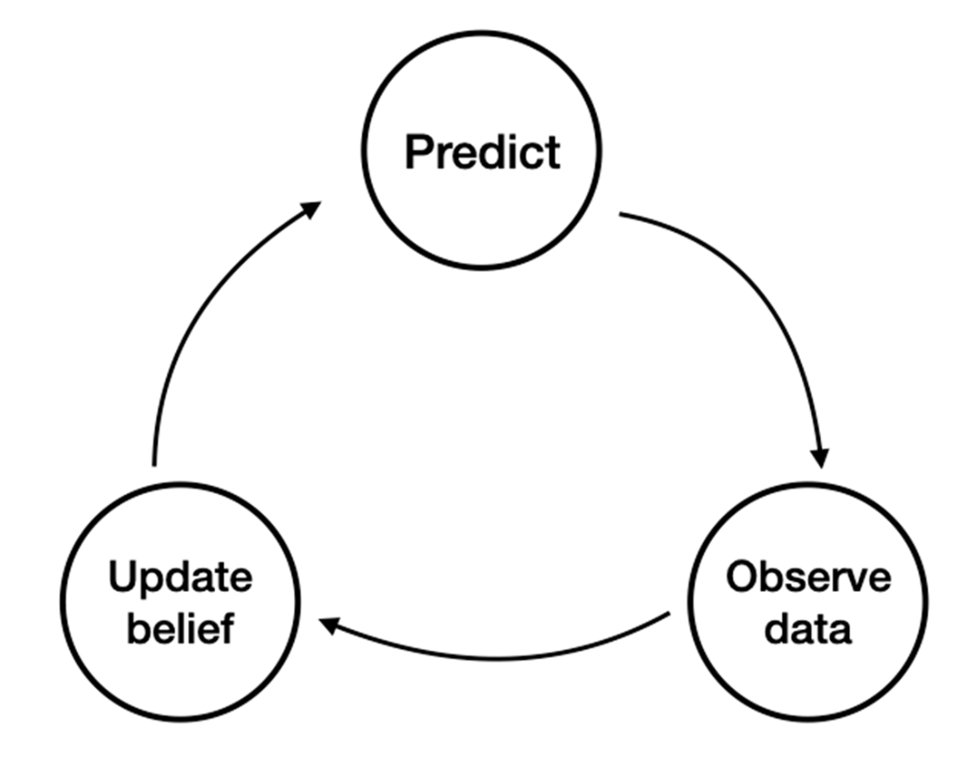
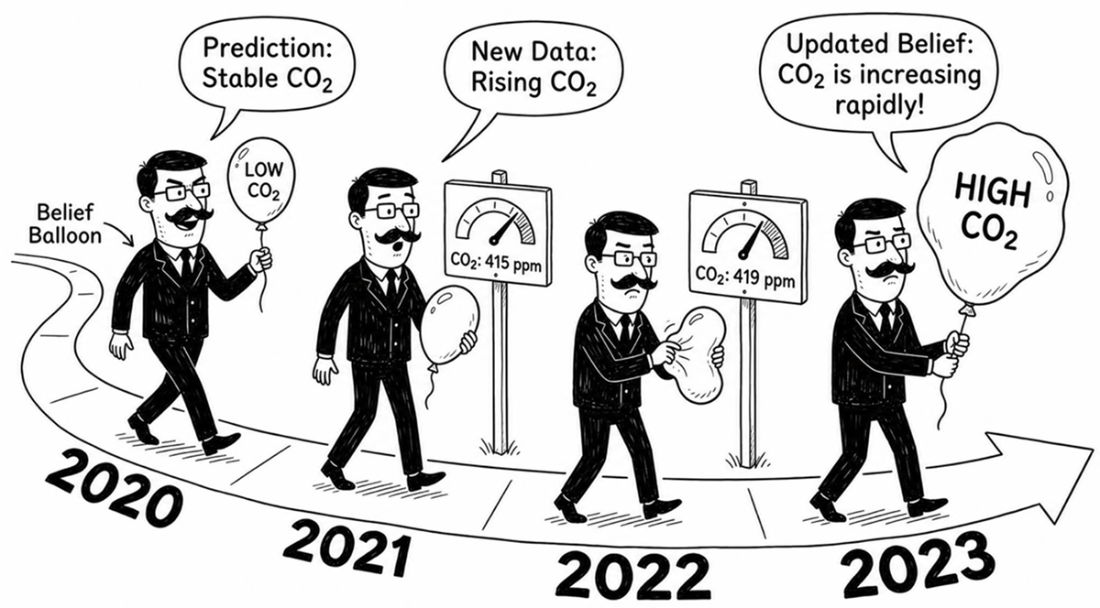
This chapter shifts Bayesian inference from a one-time update to an ongoing process that unfolds over time. Instead of learning from a complete data set all at once, it treats many problems as sequential: predictions are made, new observations arrive, beliefs are revised, and the cycle repeats. Using yearly atmospheric CO₂ measurements from Mauna Loa as a running example, it shows why time series require models that can adapt as data are revealed step by step rather than only at the end.
The key modeling idea is the state space formulation, which separates an evolving hidden state from the observations generated from it. A filter is then the recursive algorithm that estimates the hidden state using all information available so far, alternating between prediction and update. In the simplest Bayesian version, this becomes a Kalman filter under linear, Gaussian assumptions: the state is predicted forward with process noise, the observation is modeled with measurement noise, and the Kalman gain determines how much the new data should influence the updated belief.
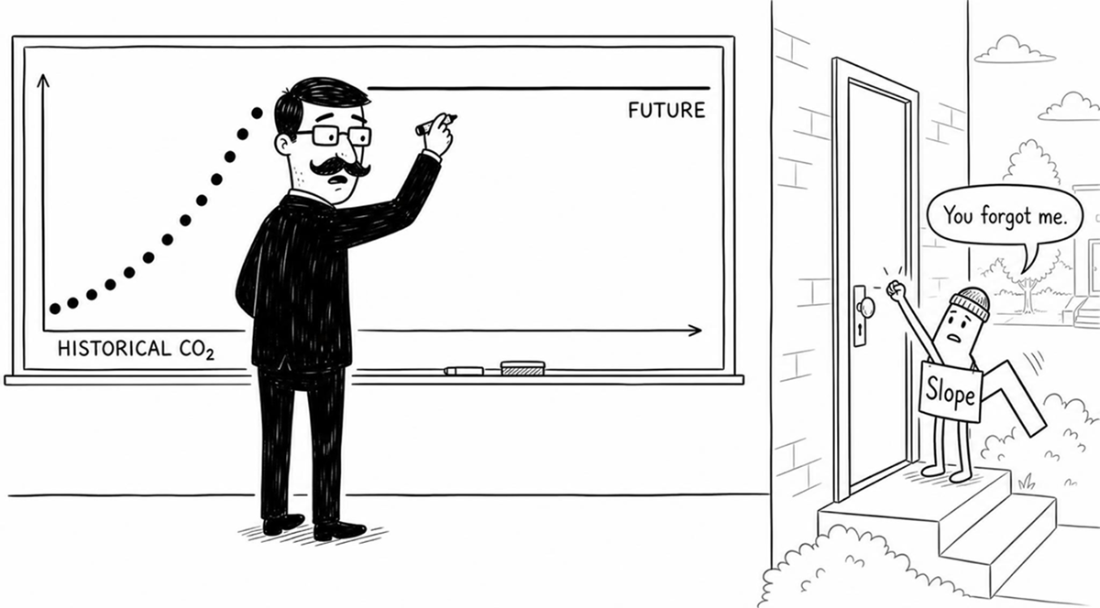
The chapter first builds a random walk filter, then shows its limitations: it can track the present reasonably well but tends to make flat long-term forecasts because it does not explicitly model trend. Increasing the state-transition variance makes the filter more flexible, but a better solution is to expand the hidden state to include both level and slope, yielding a multivariate Kalman filter that can represent a persistent upward trend in CO₂. The chapter closes by situating this framework in a broader family of filters, including extended, unscented, and ensemble Kalman filters, which adapt the same predict–update logic to nonlinear or high-dimensional real-world problems.
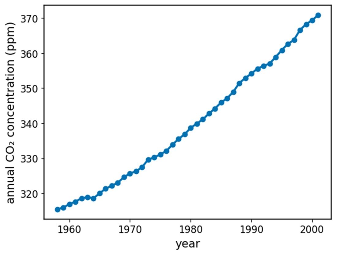
Yearly average CO₂ concentrations measured at Mauna Loa Observatory between 1958 and 2001. The time series shows an upward trend.
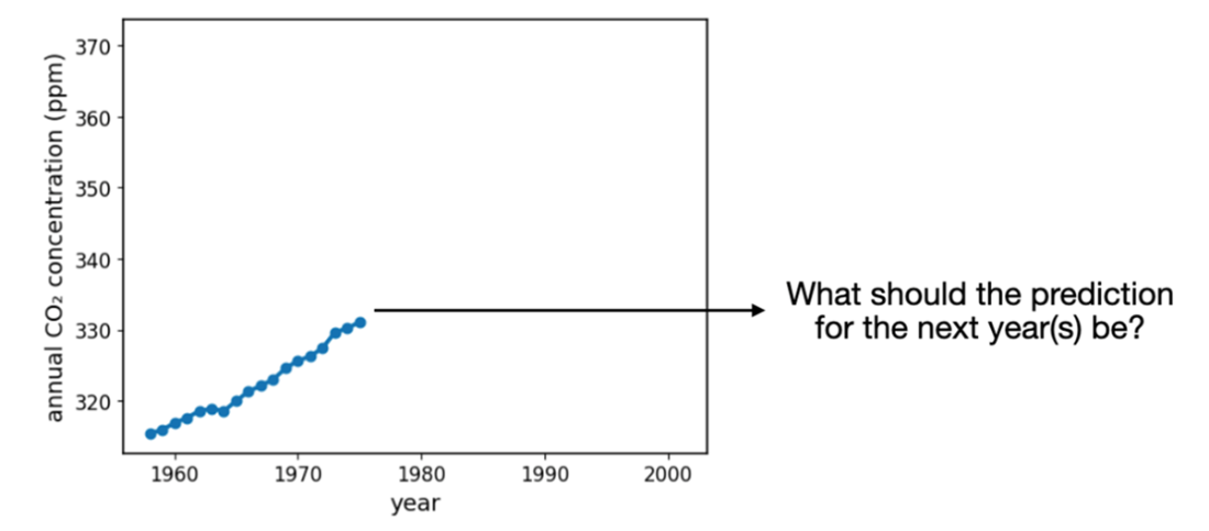
When modeling a time series, we aim to make forecasts about future data. This would require accounting for the temporal dynamics of the portion of the data we have observed.
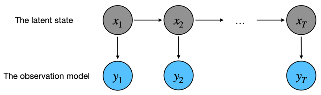
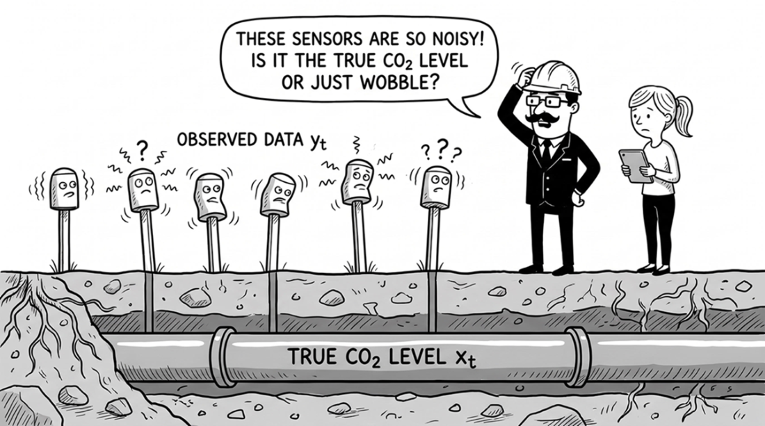
A diagram of a state space model, which includes an unknown latent space 𝑥ᵢ that evolves, and the observation model, which describes the relationship between the latent state and observed data 𝑦ᵢ at each time step.
The diagram of a filter algorithm, which alternates between the prediction step and the update step to recursively generate predictions for a time series.
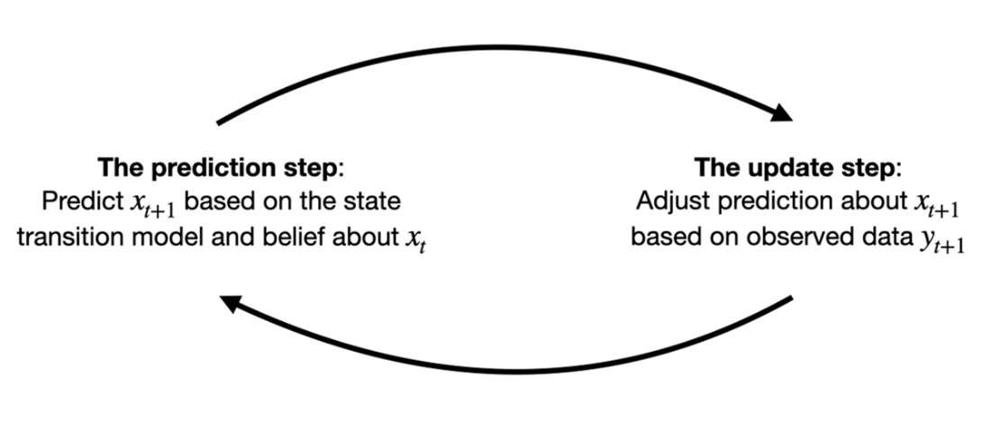
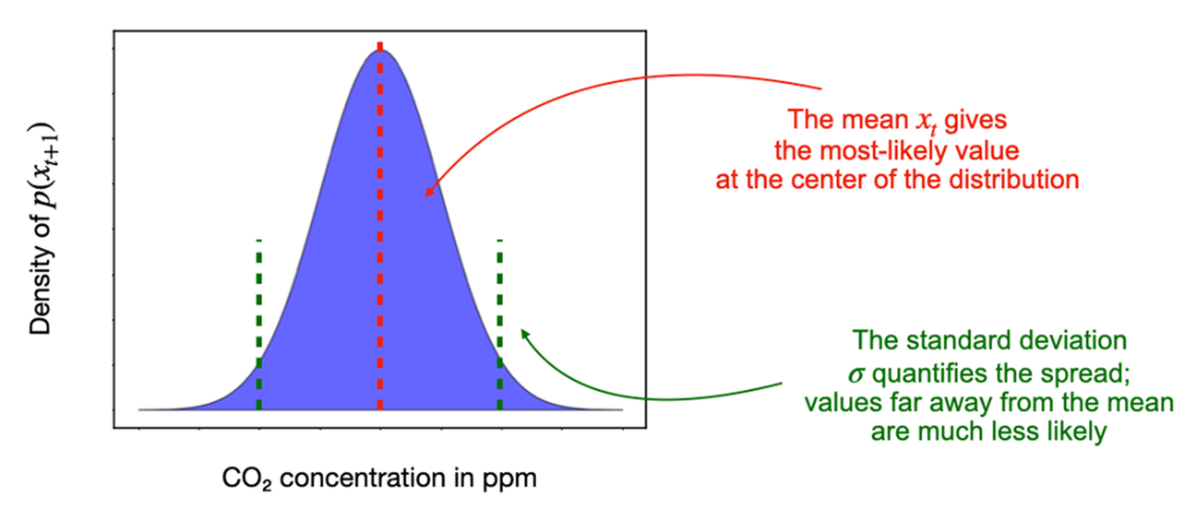
Illustration of the state transition model that assumes the next state 𝑥ᵢ₊₁ is similar to the current state 𝑥ᵢ with some zero-mean noise added.
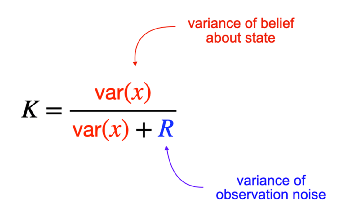
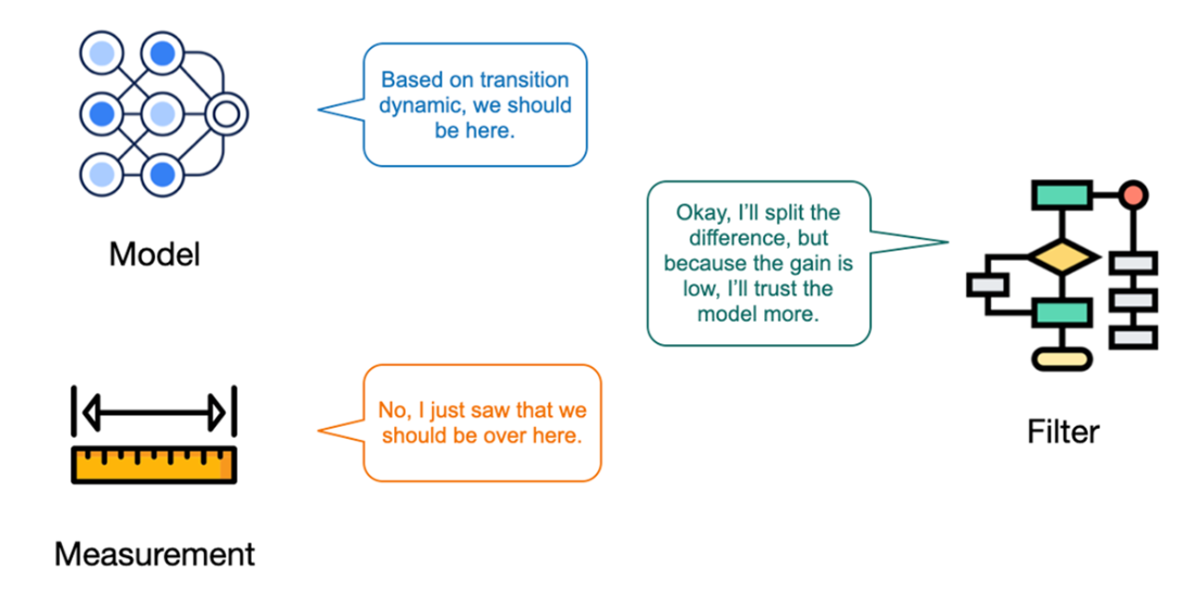
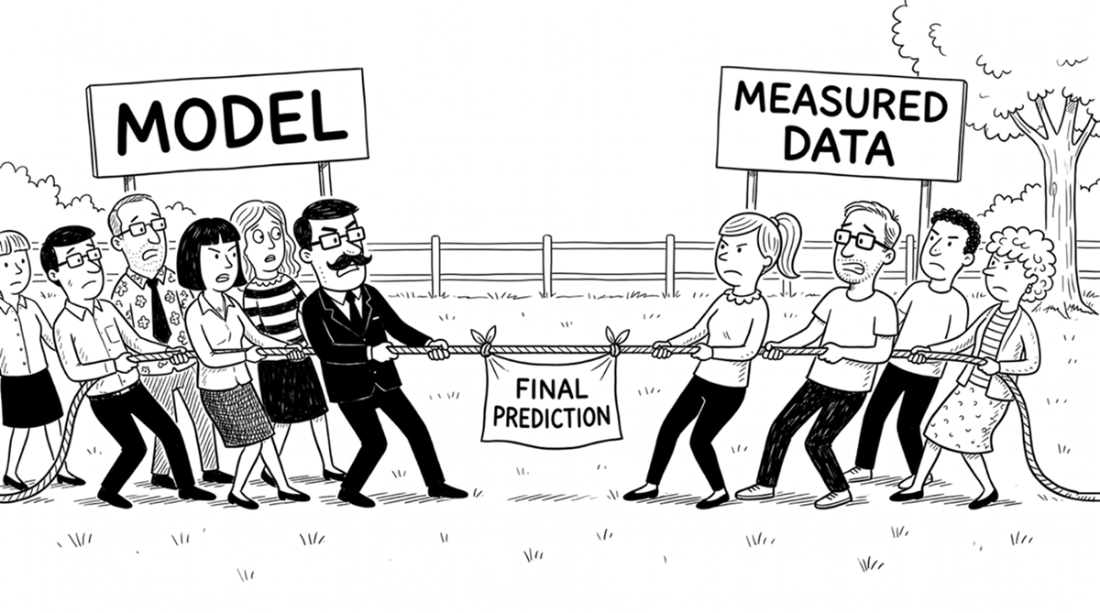
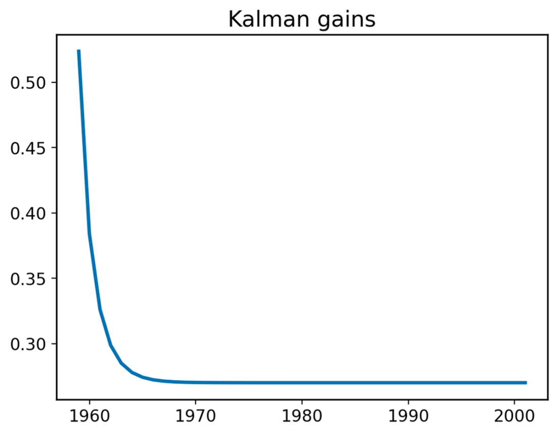
The Kalman gain helps the filter decide how much we should trust the model compared to the measurement when producing the filtered posterior prediction.
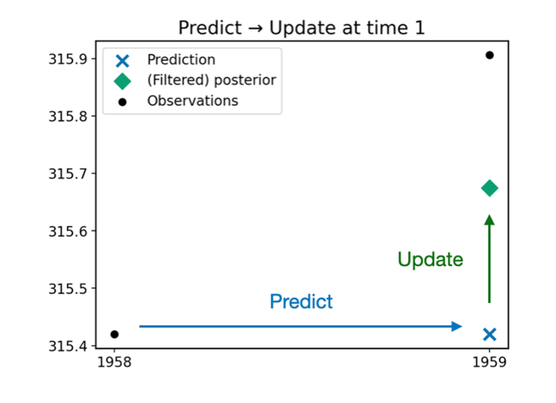
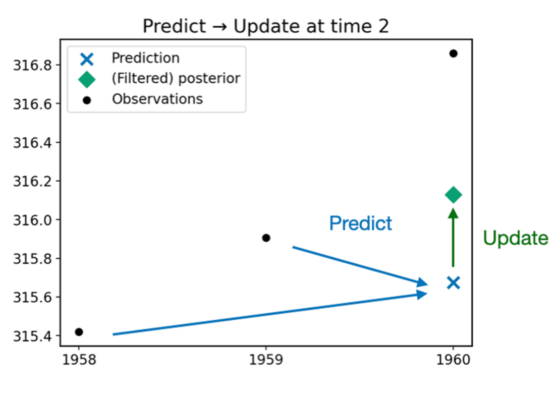
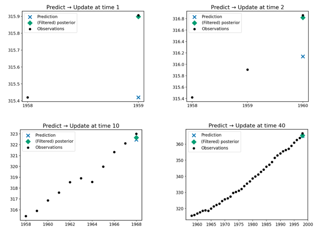
Mean predictions of the model generated at the prediction step (bottom right x) and at the update step (top right diamond) at the second time step given the observed data (dots).
Mean predictions of the model generated at the prediction step (bottom right x) and at the update step (top right diamond) at the third time step given the observed data (dots).
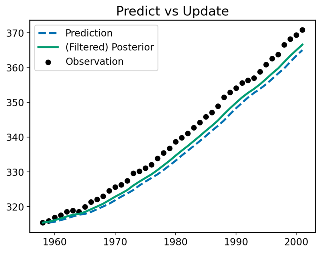
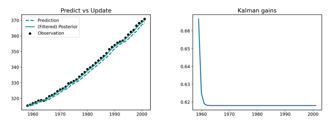
Mean predictions of the model generated at the prediction step (dashed line) and at the update step (solid line) given the observed data (dots) at each time step.
The evolution of the Kalman gain across time steps. The gain starts near 1 but quickly decreases. This trend corresponds to the filter not adjusting to observed data.
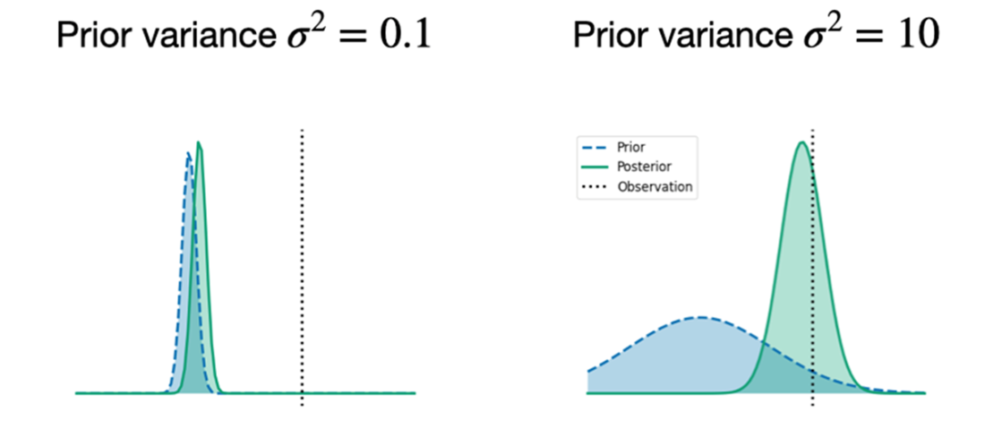
Comparison of posterior distributions adapting to data under different priors. Low prior uncertainty (small variance) leads to low adaption to data.
Behavior of the filter with a higher state transition variance, which doesn’t underestimate its predictive uncertainty and obtains higher Kalman gains. Ultimately, it adapts to observed data better than the previous filter.
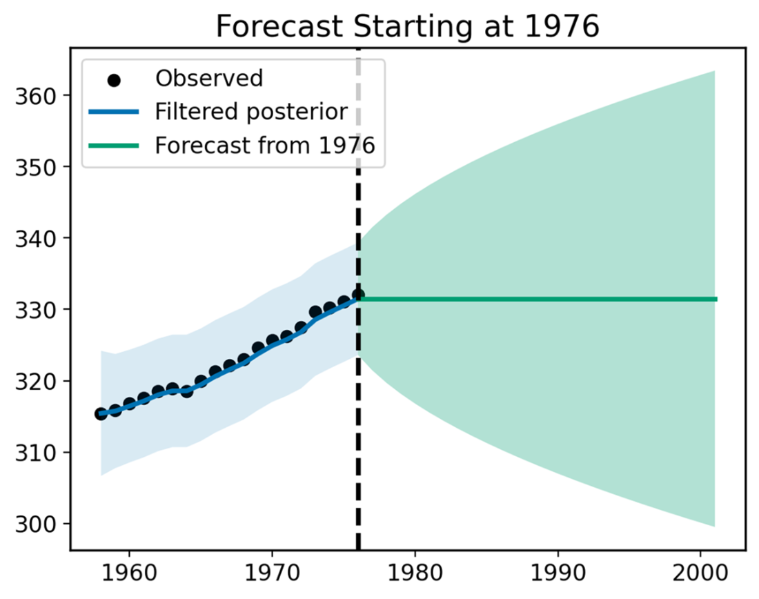
Multiyear forecasts by the random walk filter. The mean predictions stay flat as the model assumes the expected value of the latent state stays the same across time.
Mean predictions of the multivariate model generated at the prediction and update steps given the data observed at various time steps.
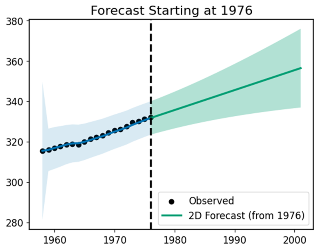
Multiyear forecasts by the multivariate filter. The mean predictions increase linearly as a function of time, as the model assumes the expected value of yearly change in CO₂ concentration to be constant.
Summary
- A state space model separates system dynamics from the observation process.
- The hidden state evolves according to a transition model; data are noisy observations of that state.
- The Kalman filter performs recursive Bayesian inference in linear Gaussian state space models.
- Filtering computes the posterior distribution of the current state given all observations so far.
- Each Kalman step consists of a prediction step that propagates the state forward and an update step that incorporates new data.
- In the linear Gaussian case, the posterior remains Gaussian; tracking the mean and covariance is sufficient.
- The Kalman gain determines how strongly new observations influence the state estimate.
- In one dimension, the Kalman gain is a scalar; in multivariate models, it becomes a vector that quantifies information across state components.
- A random walk model assumes incremental evolution with no explicit trend component.
- Forecasting propagates the state forward without incorporating new observations.
- In a random walk, multi-step forecasts have a flat predictive mean and increasing uncertainty.
- A linear trend model augments the state with a slope component.
- The Kalman filter provides a computationally efficient framework for sequential probabilistic reasoning in time-evolving systems.
- The Extended Kalman Filter handles nonlinear dynamics through local linearization.
- The Unscented Kalman Filter propagates uncertainty through nonlinear systems using deterministic sigma points.
- The Ensemble Kalman Filter approximates the posterior with a collection of state vector samples and is widely used in large-scale systems.

 Grokking Bayes ebook for free