7 Hierarchical models: Uncovering the layers of data the Bayesian way

Bayesian hierarchical models are introduced as a way to handle data that naturally comes in groups, rather than assuming every observation is drawn from one identical population. Using the example of coaching programs across eight schools, the chapter shows why treating each school completely separately can make estimates too noisy, while forcing all schools to share one effect can hide real differences. A hierarchical model sits between these extremes by letting each group have its own effect while also allowing those effects to be informed by shared structure.

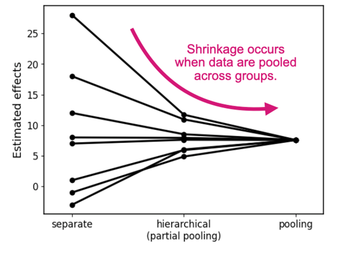
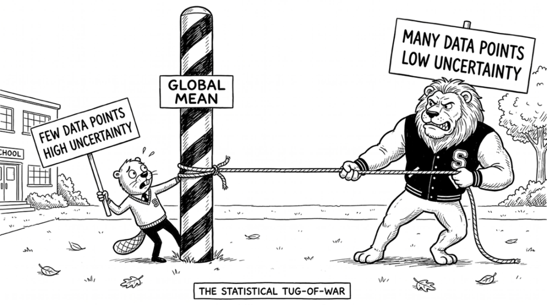
The core idea is that school-specific effects are not independent, but are drawn from a common distribution with a shared average and a spread that controls how different the groups can be. This shared structure lets information “pool” across schools, so data from one group helps stabilize estimates for the others. In the coaching example, the model estimates a positive overall effect while also allowing some schools to perform better or worse than average, with the amount of variation determined by the spread parameter.

This partial pooling produces shrinkage, meaning extreme group estimates are pulled toward the overall trend, which reduces overconfident or implausible conclusions. Compared with separate or fully pooled models, the hierarchical approach gives more balanced inferences, especially when some groups have limited data. The chapter closes by emphasizing that this framework is broadly useful beyond education, with applications in areas like sports, epidemiology, and medicine, wherever group-level variation and shared patterns both matter.

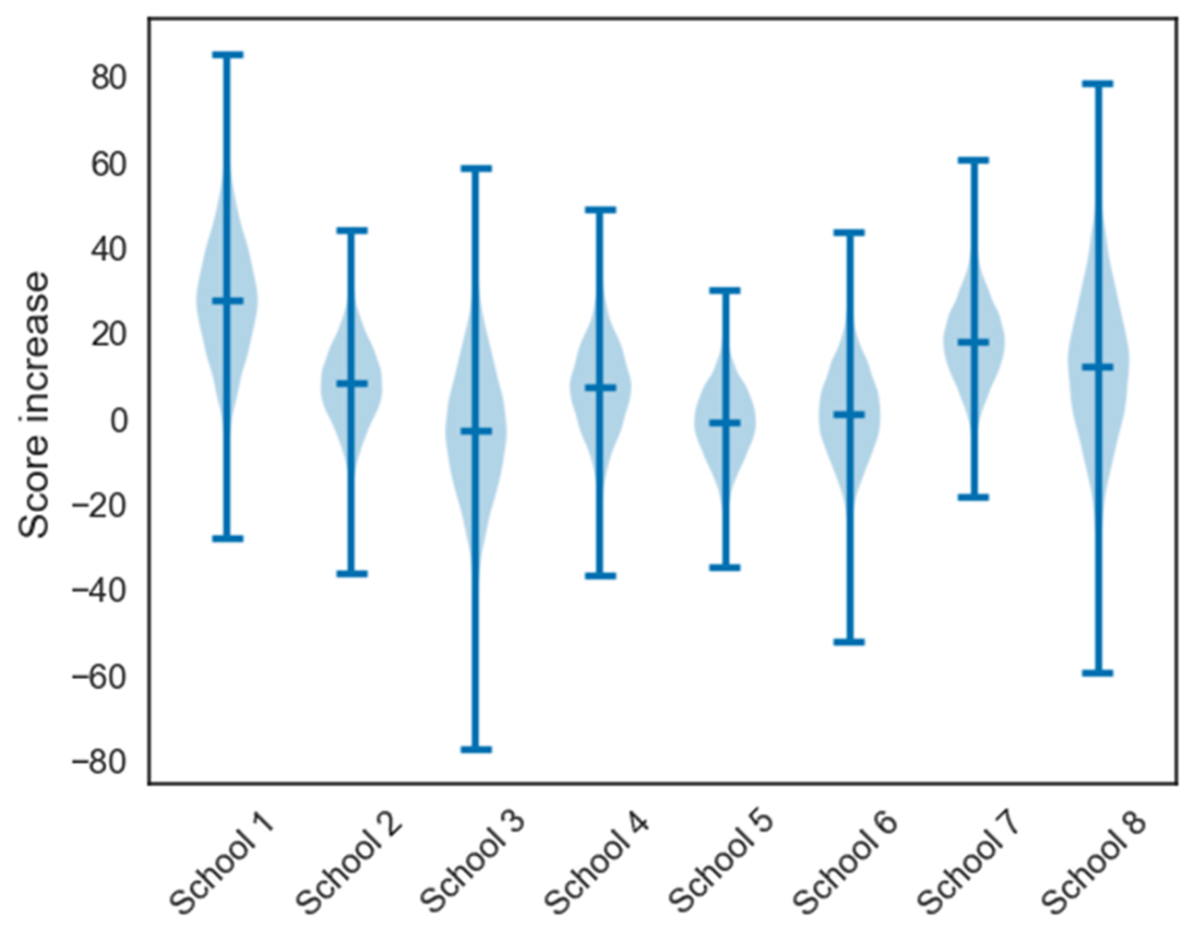
The effect of coaching in terms of increase in students’ test scores by the separate model that assumes each school makes up a unique, independent distribution.

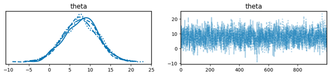
The posterior distribution of the effect of coaching under the pooled model. The effect centers around 7.7 points and ranges from −10 to 25.

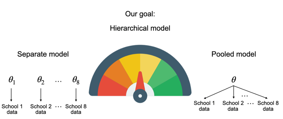
A hierarchical model is a compromise between two extremes: a separate model that doesn’t share information across the subpopulations and a pooled model that assumes there’s no heterogeneity between groups.

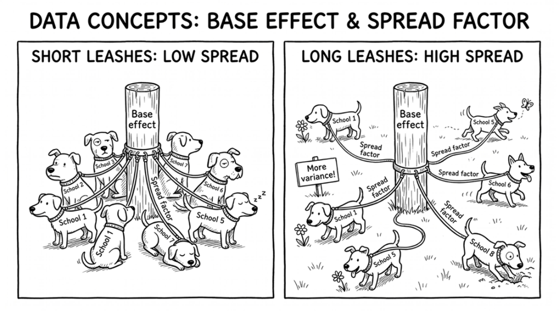
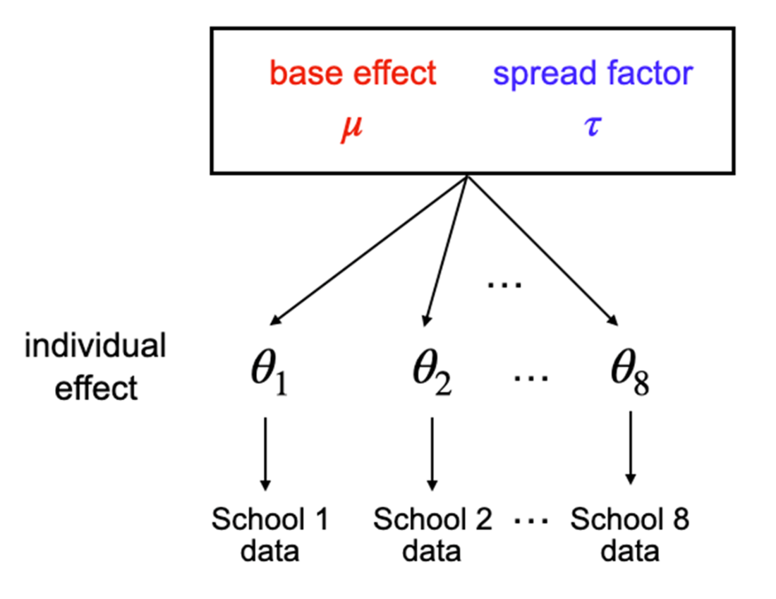
The structure of the partial pooling model, showing multiple levels of dependence between the variables involved.

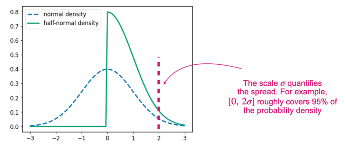
The half-normal distribution assigns probability to only half of the corresponding zero-centered normal distribution 𝒩(0, 𝜎²).

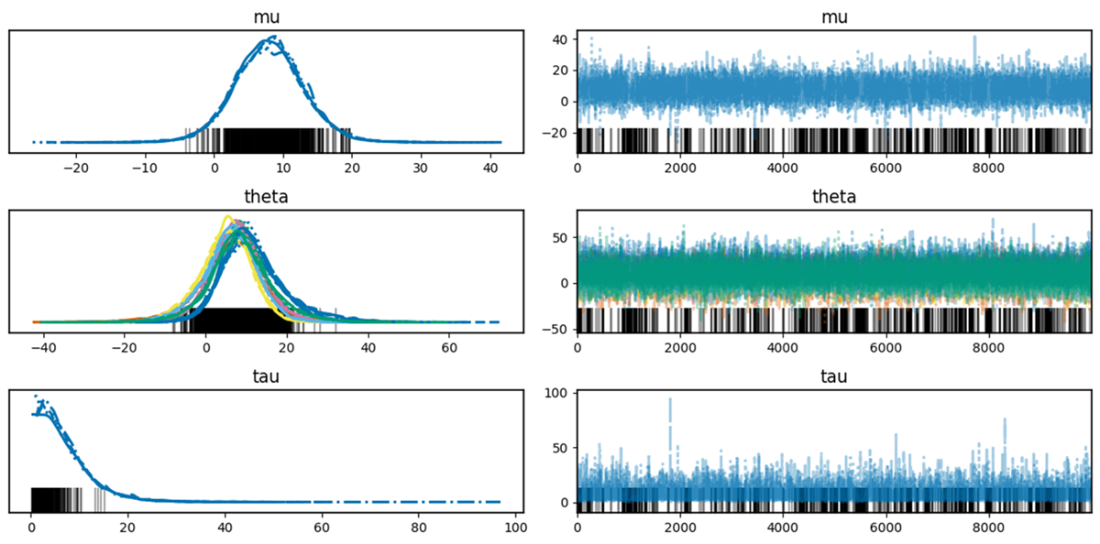
The posterior distribution of the variables in the hierarchical model. The base effect 𝜇 centers around 9, while the spread factor 𝜏 is more likely near 0. Individual effects 𝜃ᵢ are different but mostly resemble the base effect 𝜇.

Conditional average individual effect 𝐸[𝜃ᵢ | 𝜏] as a function of the spread factor 𝜏.

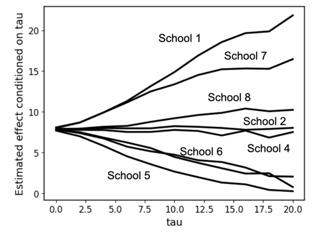
The effect of pooling in shrinking the individual effects towards a global trend.

• Hierarchical models explicitly model observations as arising from different groups that partially share common characteristics but also possess their own unique behavior. This is done by treating the statistics that describe the behavior of each group as samples drawn from a common distribution.
• Hierarchical models let us pool information across related groups while still allowing each group to have its own parameters.
• Hierarchical models solve the “all-or-nothing” choice between complete pooling (treating groups as identical) and no pooling (treating groups as totally separate).
• When the variation across groups is explicitly modeled, we can make inference about the difference in behavior between individual groups conditioned on small or large between-group variation.
• Posterior inference for hierarchical models automatically balances within-group data and across-group similarity, leading to shrinkage.

FAQ