Overview

6 Variational inference: Scaling to large datasets

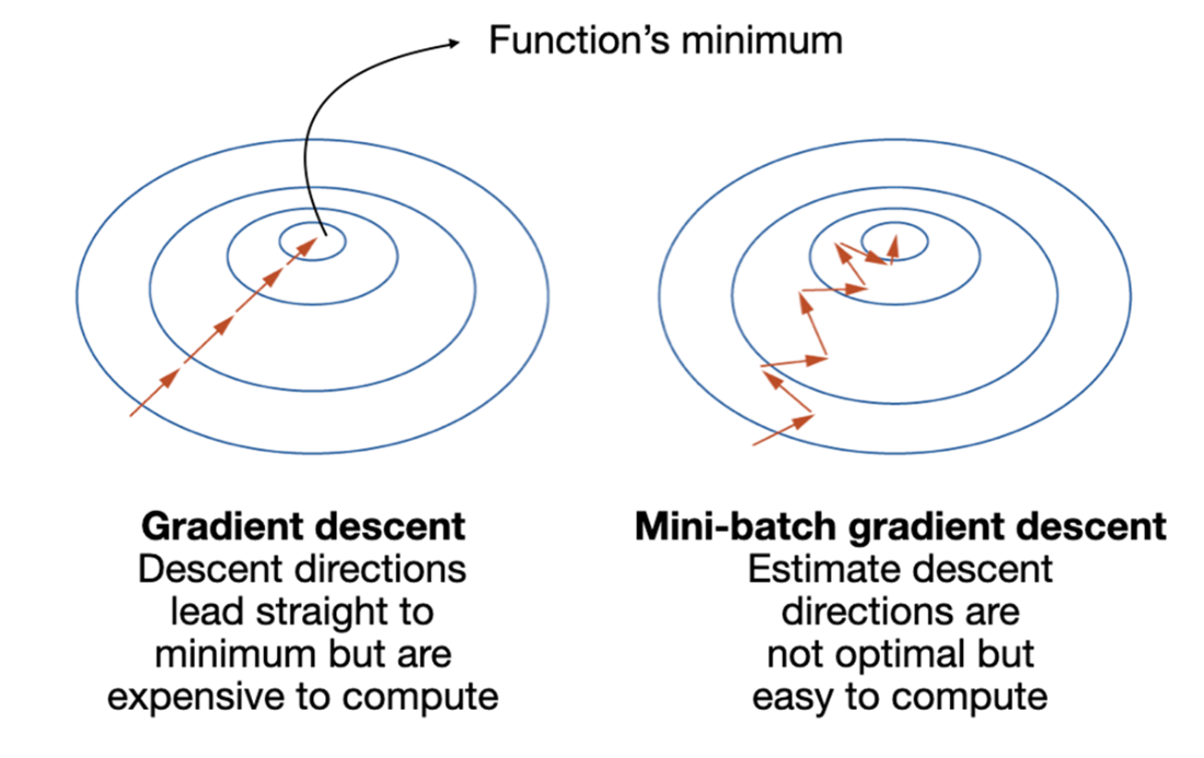
The chapter introduces variational inference as a faster alternative to MCMC for Bayesian inference on complex models and large datasets. Rather than drawing many samples from a posterior until convergence, variational inference turns inference into an optimization problem: it searches over a simple family of candidate distributions and selects the one that best approximates the true posterior. This makes it especially useful in large-scale machine learning settings where speed, frequent retraining, and real-time prediction matter.

To make this work, the chapter explains how to compare the approximating distribution to the true posterior using KL divergence, and then how to avoid directly computing that hard quantity by maximizing the ELBO instead. The ELBO reformulation uses Bayes’ theorem to express the objective in a more tractable form, allowing optimization with gradient descent. Because sampling breaks differentiability, the reparameterization trick is introduced so samples from a normal approximator can be rewritten as a deterministic transformation of a standard normal draw, restoring gradient flow and enabling automatic differentiation.

The chapter then shows how variational inference is made practical at scale through minibatch training, where each update uses a small random subset of data to estimate the ELBO and its gradient. In PyMC, fitting a variational model looks similar to MCMC, but uses a fit step and then samples from the learned approximation. The chapter closes by emphasizing that VI is usually much faster than MCMC, but often less faithful: it can miss multiple posterior modes and underestimate variance, so its quality depends on the flexibility of the approximating family and the problem at hand.

Unlike MCMC, which generates samples to approximate an unknown posterior, variational inference (VI) fits a simple distribution like a normal distribution to the posterior and uses the fitted distribution as the approximation.
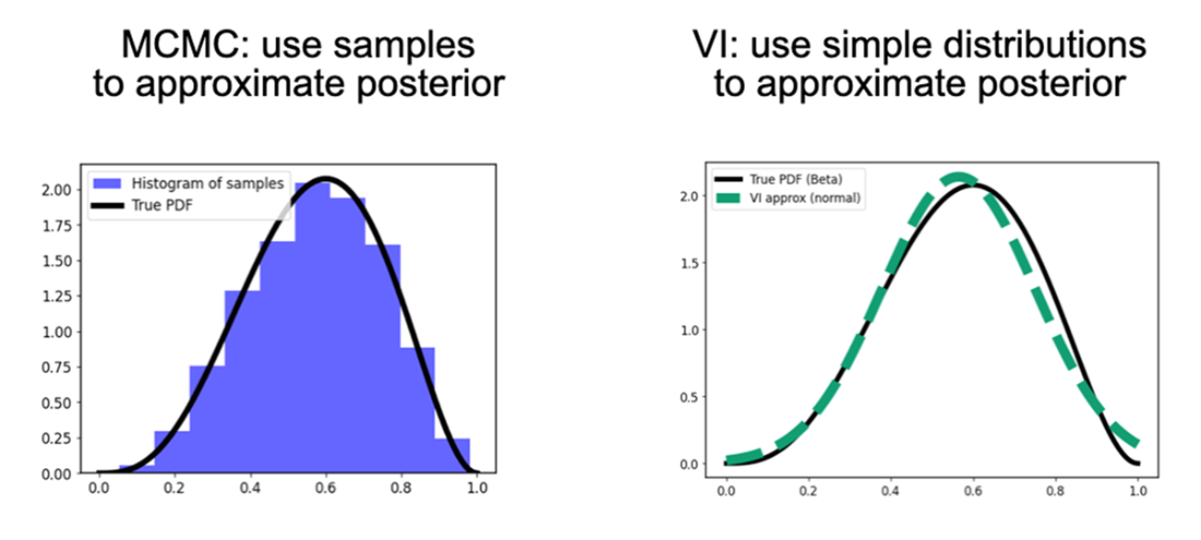
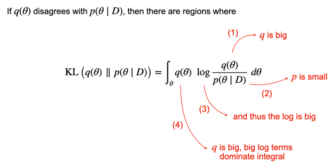
The KL divergence is large when the approximating distribution 𝑞 yields high density where 𝑝 is small. When the two distributions match, the KL divergence decreases to be close to 0.
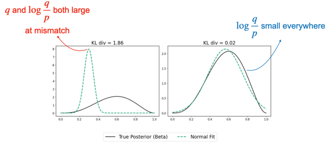
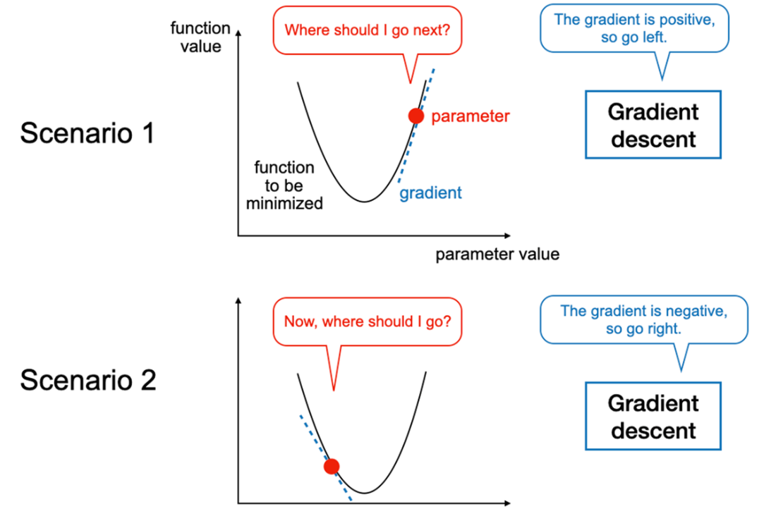
The evolution of the approximating distribution 𝑞 and how it’s adjusted by gradient descent throughout optimization.
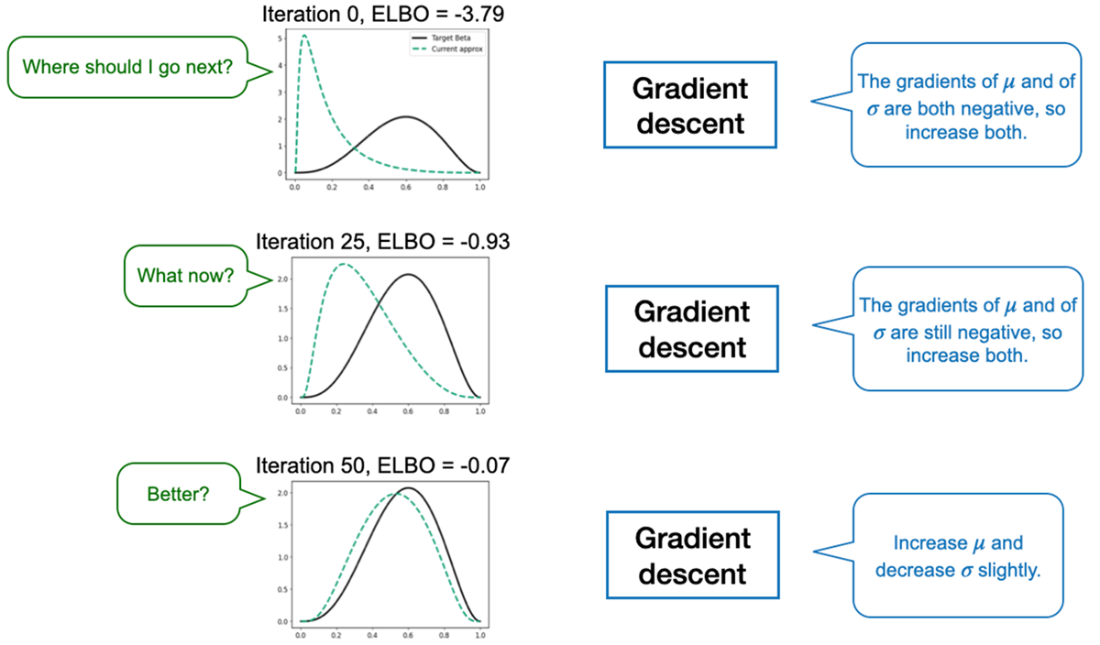
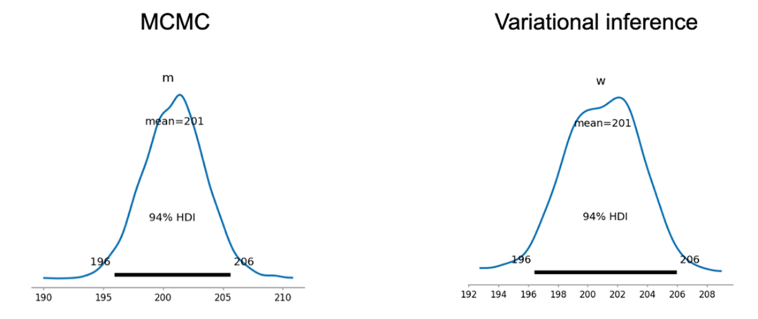
Approximate posteriors produced by MCMC (left) and variational inference (right) in the Bayesian linear regression problem. The two approximations are similar, having the same mean and 94% highest-density interval.
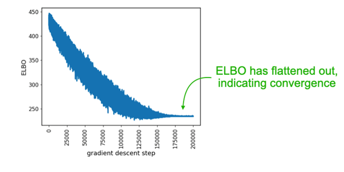
Optimization progress of the ELBO across 200,000 steps. The function’s value flattens out towards the end, indicating convergence to an optimum.
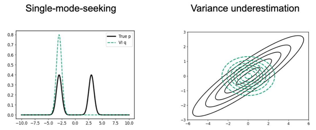
Demonstrations of pathological behaviors in variational inference. Left: mode-seeking causes the approximator to miss out on other modes. Right: variance underestimation results from the KL divergence formulation.
Summary

  • MCMC is powerful but slow, especially for high-dimensional models or large datasets.
  • Variational inference (VI) reframes inference as optimization, fitting a simple distribution to approximate the posterior.
  • The KL divergence measures the gap between the approximating distribution and the true posterior; maximizing the ELBO minimizes this gap.
  • Gradient descent with automatic differentiation makes optimization possible, but sampling blocks gradients—solved by the reparameterization trick.
  • Minibatch VI allows scaling to very large datasets, similar to how deep learning trains.
  • Pathological behaviors: VI tends to be mode-seeking and can underestimate variance due to KL’s asymmetry.
  • Advanced VI methods (mean-field, structured VI, mixtures, amortized inference, normalizing flows) extend flexibility while balancing speed.
  • MCMC vs. VI tradeoff: MCMC is slower but more faithful; VI is faster but approximate. Our choice is based on dataset size and inference needs.

FAQ

What is variational inference in Bayesian modeling?Variational inference is an optimization-based way to approximate a posterior distribution. Instead of sampling from the posterior like MCMC, it chooses a simple family of distributions and finds the member of that family that is closest to the true posterior.
Why is variational inference often faster than MCMC?VI is faster because it turns inference into an optimization problem over a simple distribution, which can be solved efficiently with gradient-based methods. It can also use minibatches, making it scalable to large datasets and high-dimensional models.
What problem does the Kullback–Leibler (KL) divergence solve in VI?The KL divergence measures how different the approximating distribution q is from the true posterior p. In VI, we minimize KL divergence so that q becomes as close as possible to p.
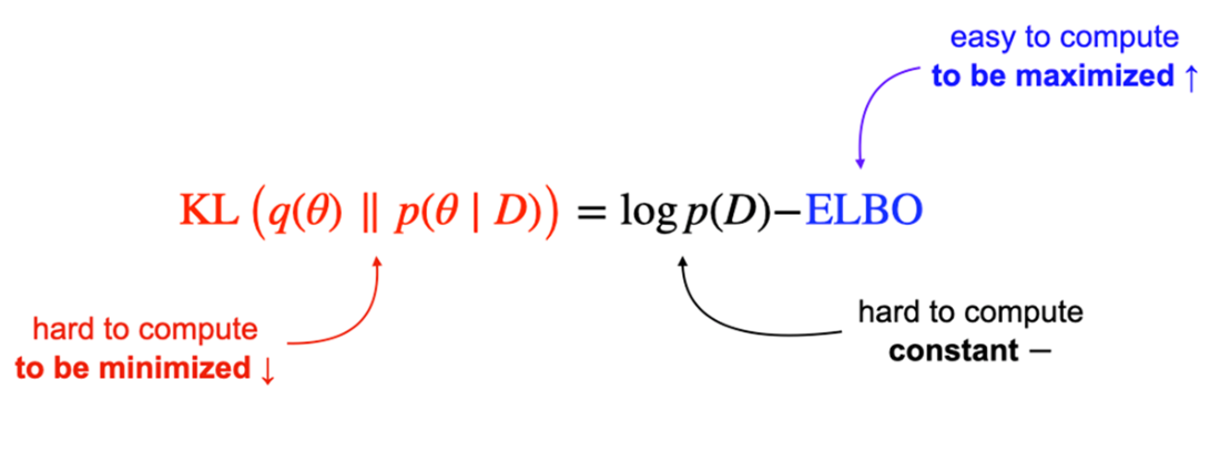
What is the ELBO and why is it important?The ELBO, or Evidence Lower Bound, is a quantity that is easier to compute than the KL divergence directly. Maximizing the ELBO is equivalent to minimizing the KL divergence between q and the posterior, so it becomes the practical objective in VI.
Why can’t we compute the KL divergence directly?Directly computing the KL divergence requires knowing the true posterior p(θ|D), which is usually intractable. The ELBO trick rewrites the problem so we can optimize using quantities that are computable, like the unnormalized posterior and q.
What is the reparameterization trick?The reparameterization trick rewrites a random sample from q as a deterministic function of a fixed noise distribution and the parameters of q. For a Normal q, a sample can be written as θ = μ + σε, where ε ~ N(0,1), which allows gradients to flow through the sampling step.
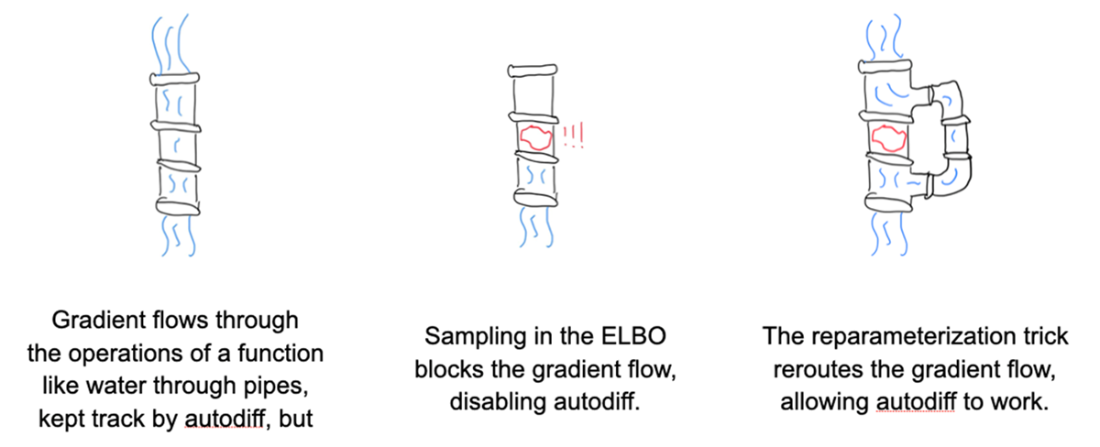
Why is the reparameterization trick needed for gradient descent?Sampling is not differentiable, so autodiff cannot compute gradients through a direct random draw. Reparameterization removes that obstacle by expressing sampling as differentiable operations on fixed noise, enabling gradient-based optimization of the ELBO.
What is minibatch variational inference?Minibatch VI estimates the ELBO and its gradient using a small random subset of the data rather than the full dataset. This reduces computation and memory use, making VI practical for very large datasets.
What are the main limitations of variational inference?VI can be biased because the quality of the approximation depends on the chosen family q. Simple choices like a Normal distribution may miss multimodality, underestimate variance, or fail to capture correlations in the true posterior.
When should I use variational inference instead of MCMC?Use VI when speed and scalability matter most, especially for large datasets, real-time systems, or models with many parameters. Use MCMC when you need higher-fidelity posterior approximations and can afford the extra computation.

pro $24.99 per month

  • access to all Manning books, MEAPs, liveVideos, liveProjects, and audiobooks!
  • choose one free eBook per month to keep
  • exclusive 50% discount on all purchases
  • renews monthly, pause or cancel renewal anytime

lite $19.99 per month

  • access to all Manning books, including MEAPs!

team

5, 10 or 20 seats+ for your team - learn more


choose your plan

team

monthly
annual
$49.99
$499.99
only $41.67 per month
  • five seats for your team
  • access to all Manning books, MEAPs, liveVideos, liveProjects, and audiobooks!
  • choose another free product every time you renew
  • choose twelve free products per year
  • exclusive 50% discount on all purchases
  • renews monthly, pause or cancel renewal anytime
  • renews annually, pause or cancel renewal anytime
  • Grokking Bayes ebook for free