5 Monte Carlo methods: Inference by sampling: Being a tour guide for unknown Bayesian posteriors
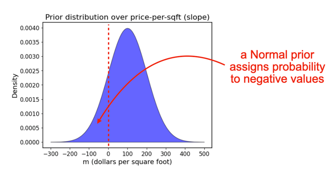
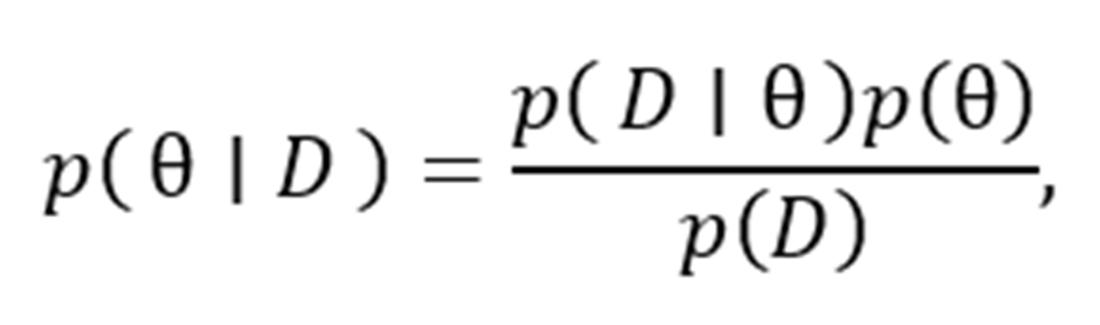
When Bayesian models are built with conjugate priors, the posterior can often be written in closed form and summarized directly with quantities like the mean or credible intervals. But real problems frequently use priors that better match domain knowledge, and those priors may break conjugacy, leaving a posterior that can be described mathematically but not solved exactly. In those cases, the key challenge is that the normalizing constant in Bayes’ rule becomes difficult or impossible to compute, so the chapter motivates a shift from analytic inference to sampling-based inference.
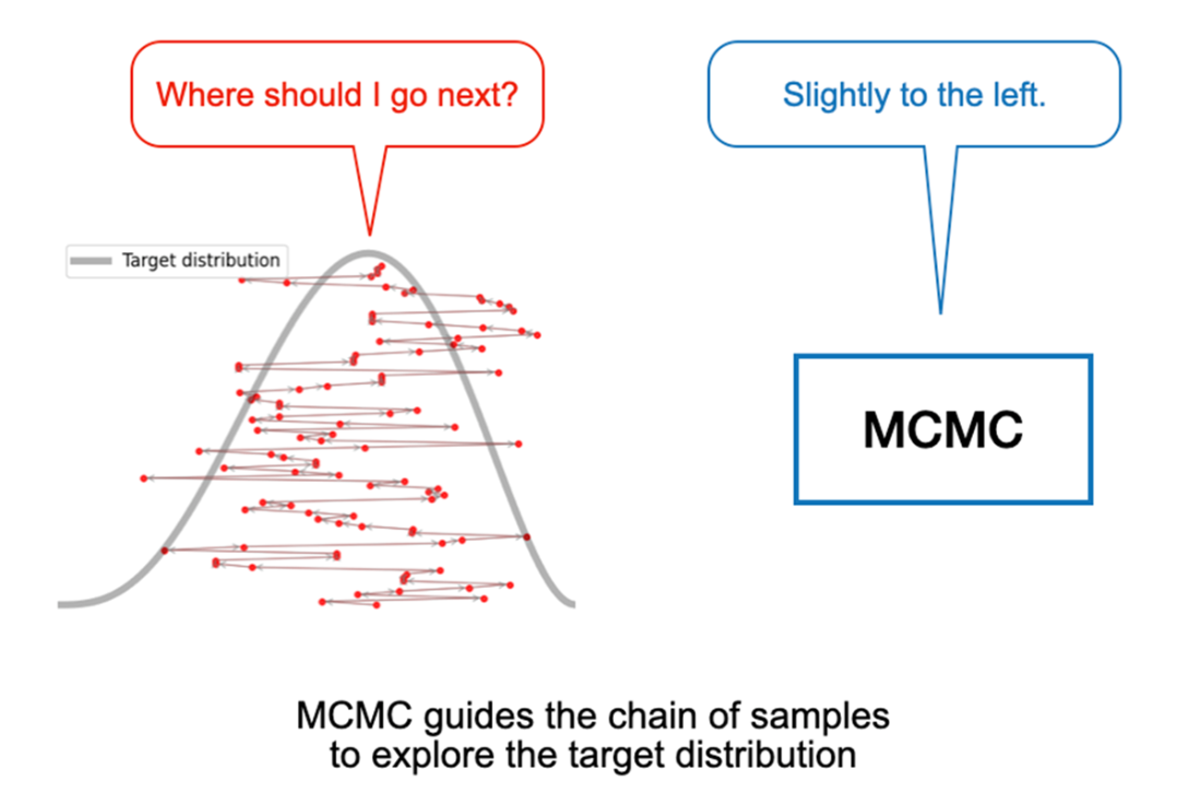
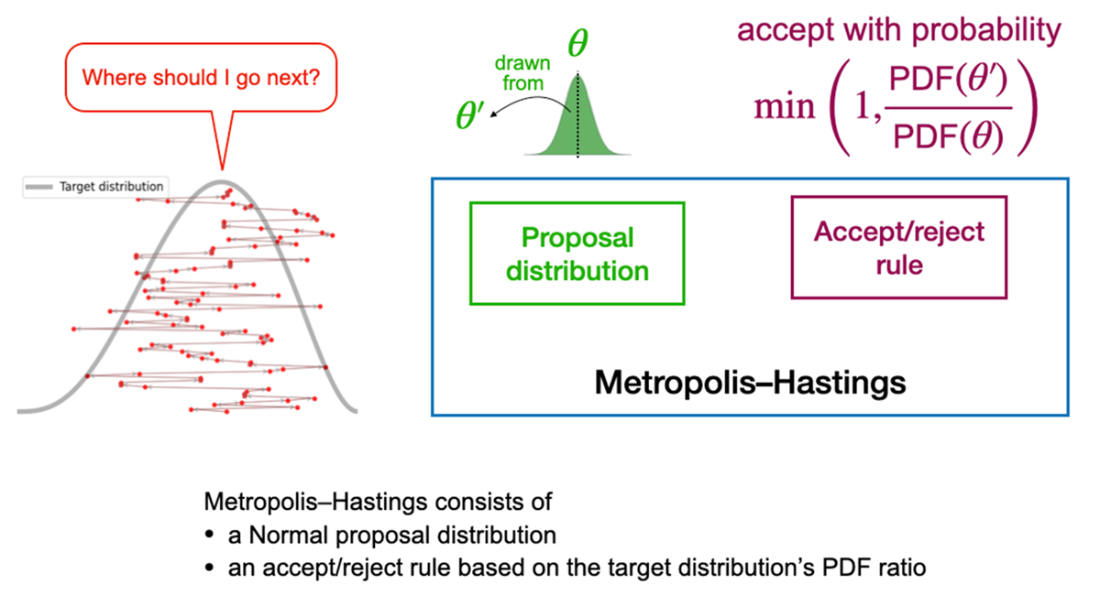
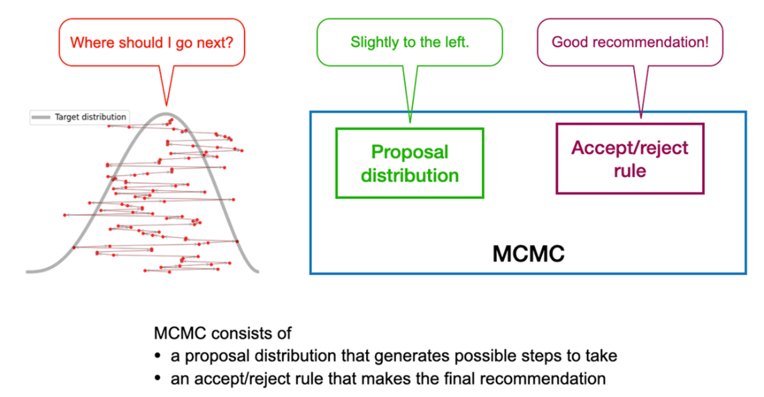
The main idea is to approximate an unknown posterior by generating samples from it and treating those samples as a stand-in for the distribution itself. With enough samples, simple statistics from the sample set can estimate posterior means, credible intervals, cumulative probabilities, and predictive behavior. This leads naturally to Markov chain Monte Carlo, which creates a dependent sequence of samples that still spends time in regions of the parameter space in proportion to posterior density. The chapter introduces the Metropolis–Hastings algorithm as a concrete example: propose a nearby move, compare unnormalized posterior densities, and accept or reject the move so the resulting chain explores the target distribution efficiently.
The chapter also emphasizes that MCMC is only useful when handled carefully. Early samples may be unrepresentative, so burn-in should be discarded, and multiple chains should be run to reduce the risk of getting stuck in poor regions. Convergence diagnostics such as R-hat and effective sample size help assess whether the chains have stabilized and whether the samples are informative enough, while trace plots reveal whether the chain is mixing well. Finally, posterior predictive checks ensure that the fitted model actually reproduces observed data plausibly. Using PyMC and ArviZ, the chapter shows how these ideas come together in practice to make sampling-based Bayesian inference usable and reliable.

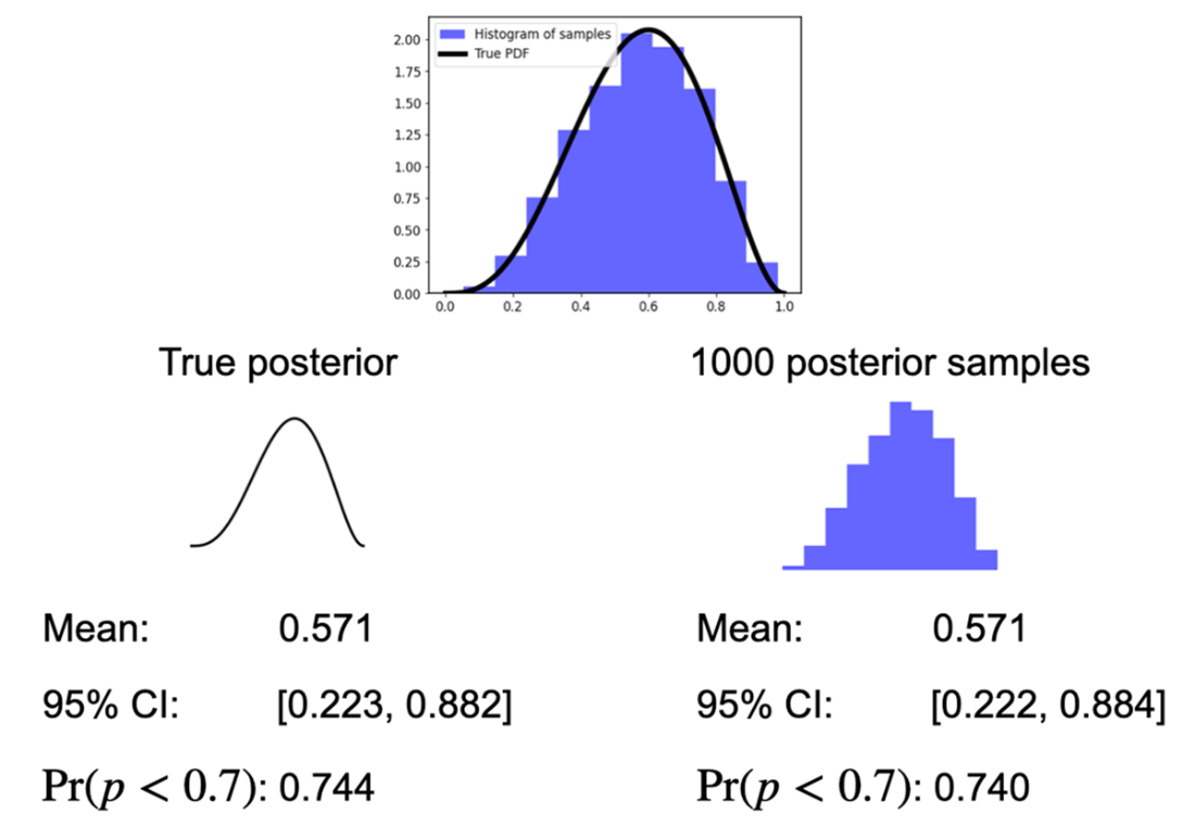
Comparison between a posterior distribution available in closed form and Monte Carlo samples. The samples’ histogram matches the true PDF, and the various statistics from the samples give reasonable approximations to the corresponding true quantities.
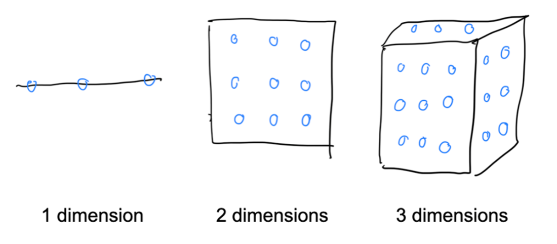
We need exponentially more samples for a grid approximation as the dimensionality grows.
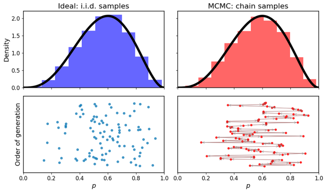
Differences between i.i.d. sampling (left) and MCMC (right). MCMC generates a chain of dependent samples (order indicated by arrows) that approximates the distribution.
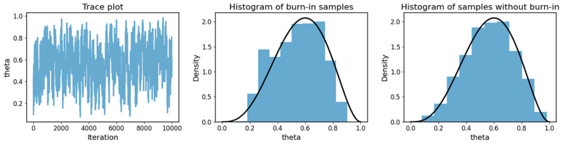
Comparison between samples during and after the burn-in period. Burn-in samples might not represent the target distribution well, so we should remove these initial samples prior to any subsequent analysis.
Various statistics describing the posterior samples generated by PyMC. The R̂ statistic at the end indicates that our MCMC chains have converged, while ESS statistics tell us about the effective sample size.

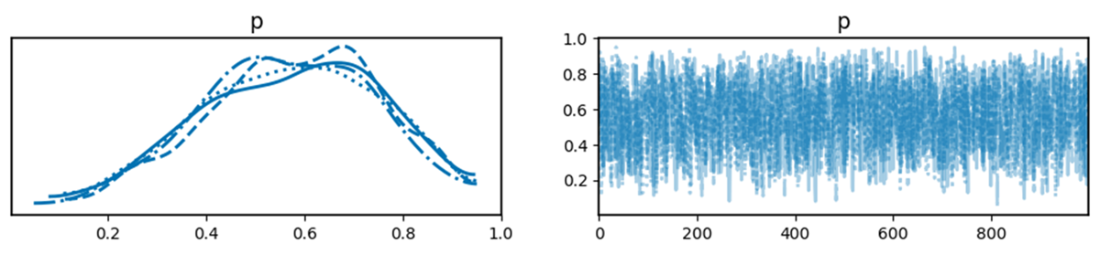
Left: the distribution of the posterior samples of 𝑝 from the four chains. Right: The trace plot of these chains, which shows hairy caterpillar patterns indicating good mixing.
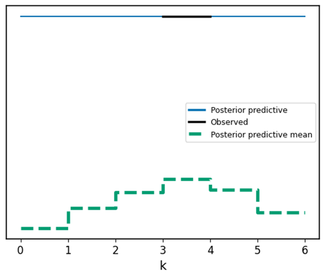
Posterior predictive check plot generated by ArviZ. The observed data lies inside the range simulated by the posterior predictive samples, indicating that our model passes the posterior predictive check.
Summary
- Monte Carlo (MC) methods approximate posteriors by generating samples instead of deriving them analytically.
- Conjugate priors allow exact posteriors, but many real-world problems require non-conjugate priors that make closed-form solutions impossible.
- MC sampling works even when we know only the unnormalized posterior, allowing us to compute statistics like means, credible intervals, and tail probabilities.
- Independent and identically distributed (i.i.d.) samples are the gold standard, but are unavailable when the posterior is not analytically tractable; Markov chain Monte Carlo (MCMC) generates dependent samples that still approximate the target.
- Grid approximation works only in low dimensions and wastes computation on low-density regions.
- MCMC uses a chain of dependent samples to efficiently explore the posterior’s high-density regions.
- Metropolis–Hastings builds this chain by proposing moves from a proposal distribution and accepting/rejecting based on posterior density ratios.
- Discarding burn-in MCMC samples removes bias from poor starting points.
- Running multiple MCMC chains avoids dependence on any single initialization.
- We can assess MCMC convergence using R̂ (close to 1) and sampling efficiency using ESS (at least 400 for bulk and tail).
- When checking mixing via trace plots, look for “hairy caterpillars,” not flat lines or jumps.
- Perform posterior predictive checks to ensure simulated data matches observed data.
- PyMC provides simple, readable syntax and integrates tightly with ArviZ for diagnostics and visualization.

 Grokking Bayes ebook for free
