3 Conjugate priors for closed-form Bayesian updates: Skipping over heavy computations with clever math

In this chapter, the focus shifts from a discretized Bayesian view of uncertainty to a continuous one, where a quantity like the office tea-preference rate can take any value between 0 and 1. The key challenge is that continuous hypotheses cannot be handled by simply assigning probabilities to finitely many cases, so the chapter introduces probability densities, integrals, and the idea that only ranges of values have meaningful probability. This sets up a more accurate and flexible version of Bayesian updating while keeping the same core logic: start with a prior belief, combine it with data through a likelihood, and update to a posterior.

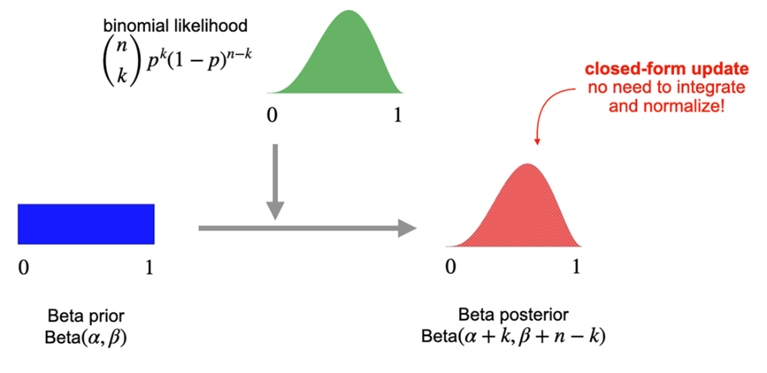
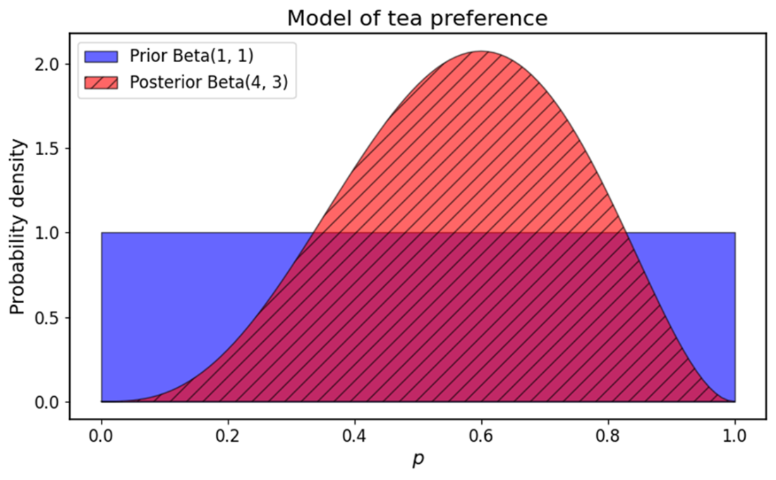
The main mathematical shortcut is the use of conjugate priors, distributions that produce posteriors from the same family and therefore avoid heavy computation. For proportions, the beta distribution pairs naturally with the binomial likelihood, making the prior update especially simple: the prior hyperparameters are incremented by observed successes and failures. The chapter uses the tea-versus-coffee example to show how a Beta(1,1) prior updated with 3 tea drinkers out of 5 becomes Beta(4,3), and explains how different beta priors encode different strengths of belief, from near-indifference to strong prior conviction.

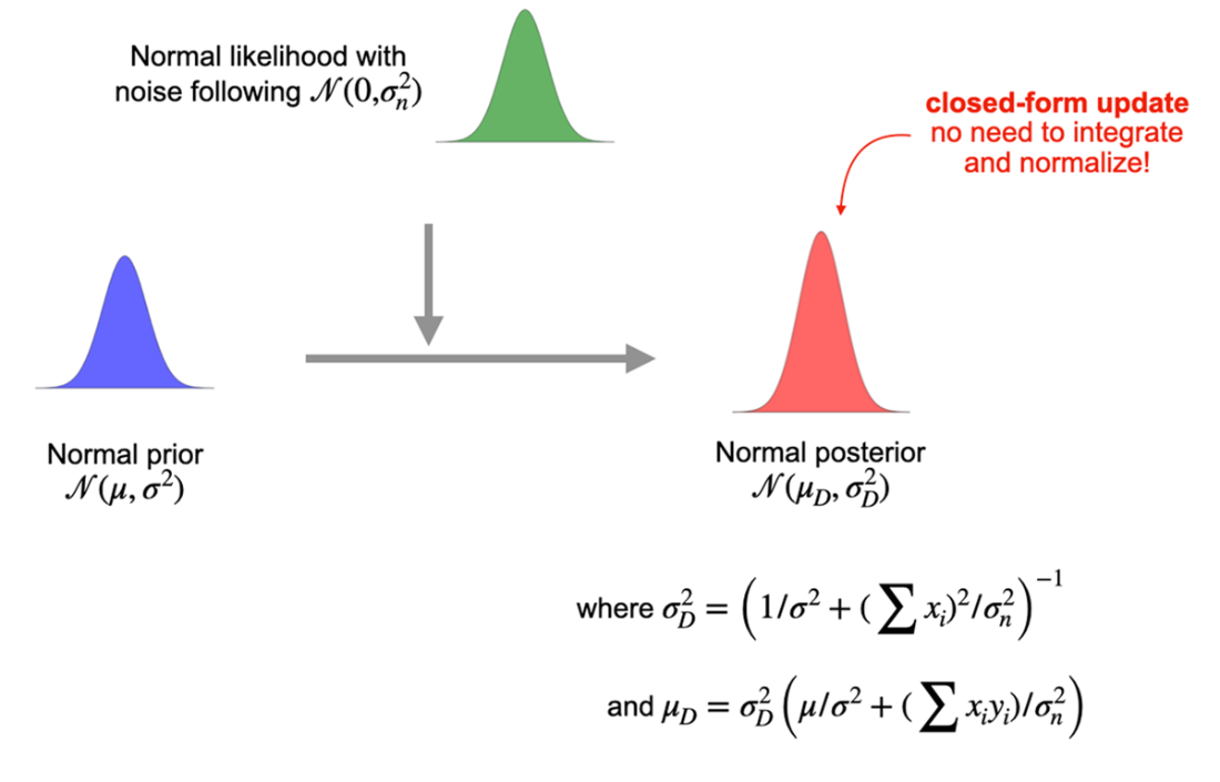
The second major application is Bayesian linear regression, where a normal prior on the slope combines with a normal noise model to yield a normal posterior over the slope and a posterior predictive distribution over future house prices. This provides not just a best estimate but also uncertainty bounds, typically expressed as credible intervals, and it connects Bayesian priors to regularization by showing that stronger priors restrain overly large weights. The chapter ends by situating these ideas in a broader landscape of conjugate models, including the Dirichlet for multinomial outcomes and the Gamma for event rates, emphasizing that conjugate priors make Bayesian inference both practical and interpretable.

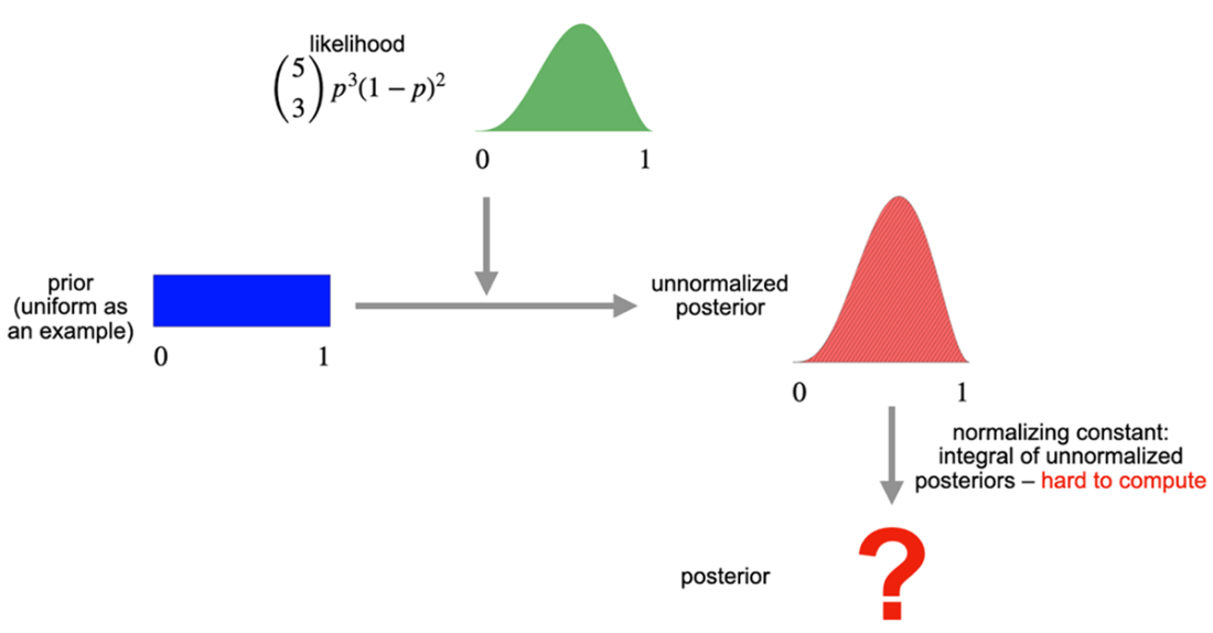
The procedure of deriving the posterior distribution under a Bayesian model: the prior is multiplied with the likelihood to produce the unnormalized posterior probabilities. These values are then normalized so that they sum to 1 to yield the posterior probabilities.

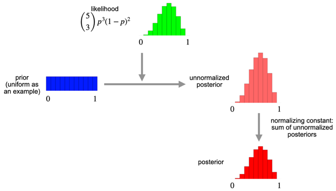
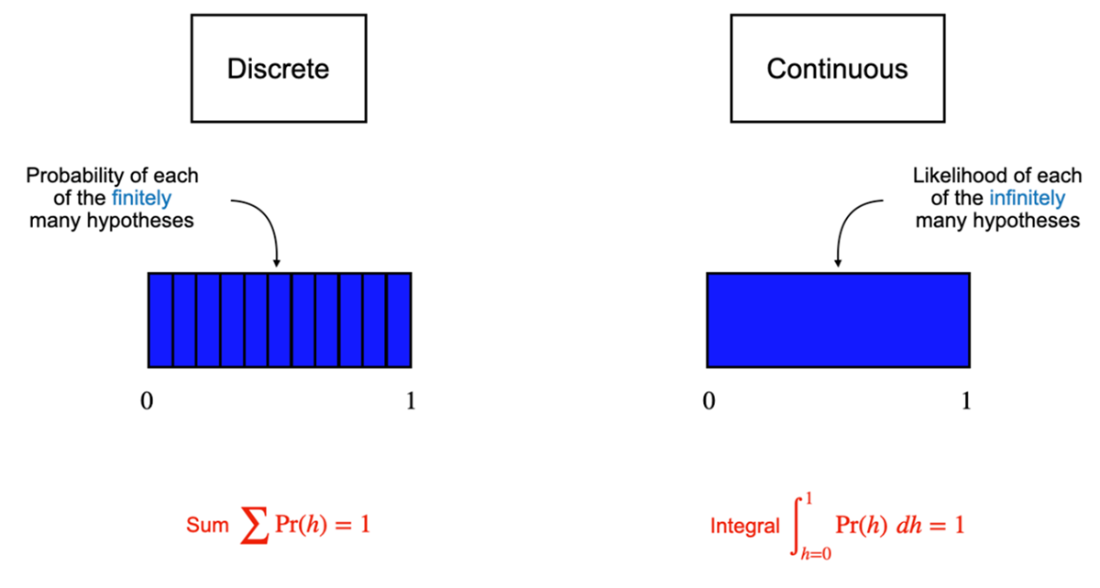
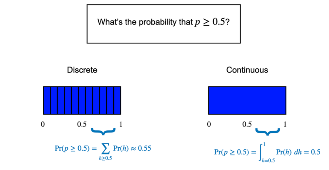
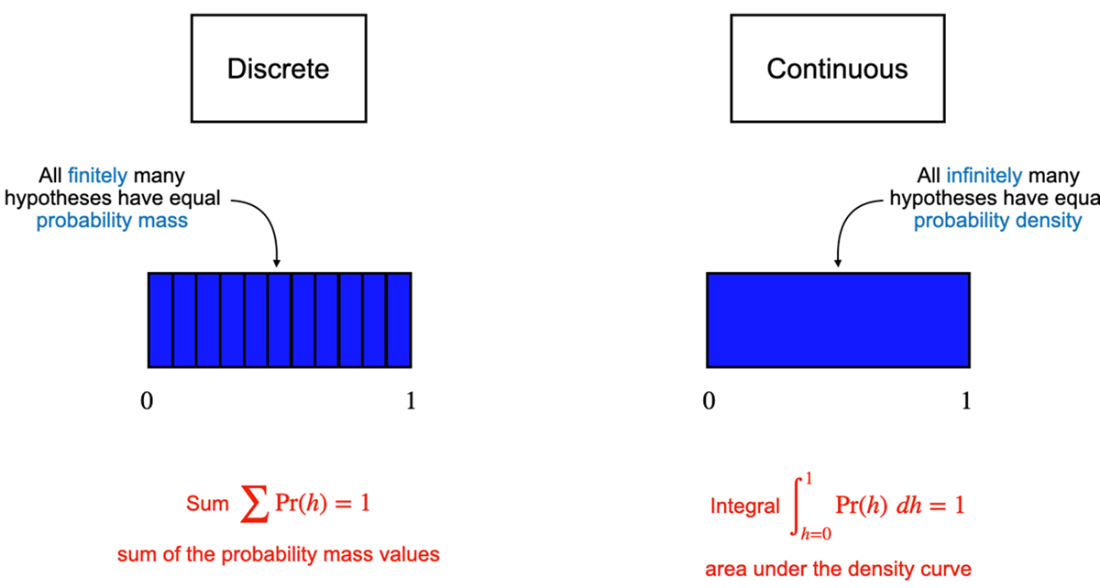
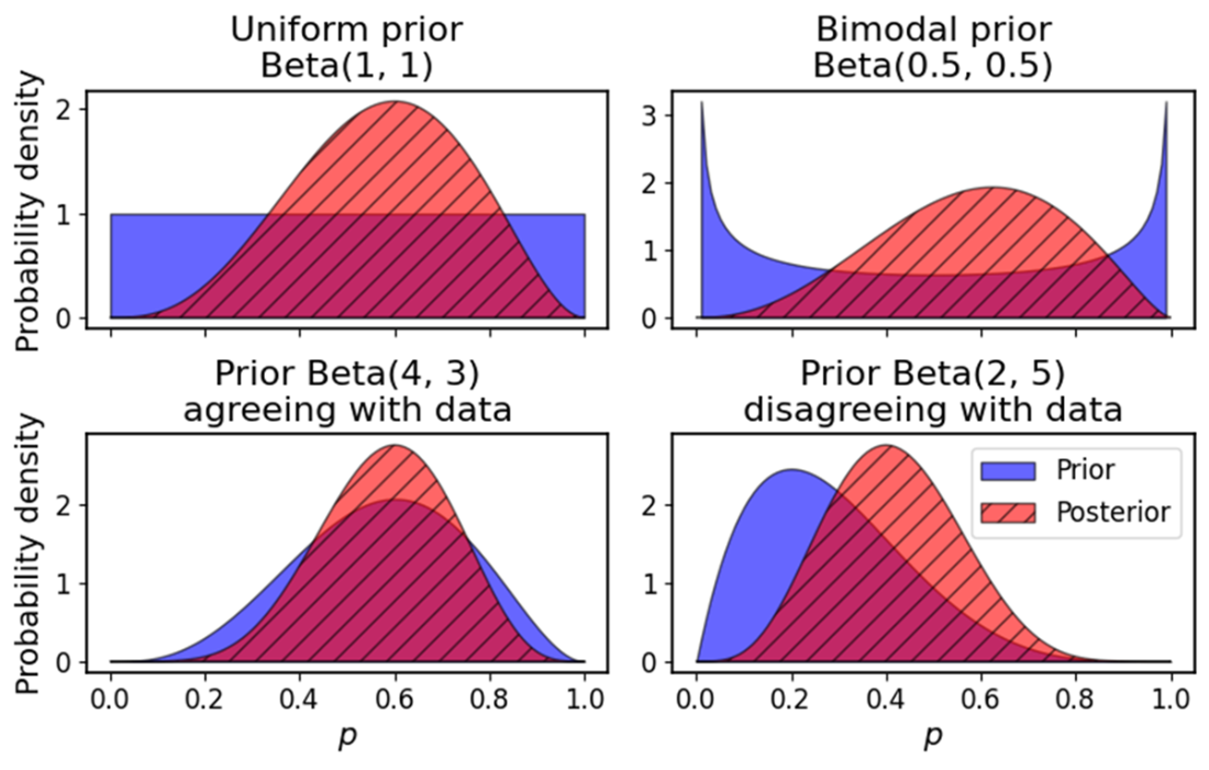
Prior and posterior probability distributions of 𝑝, the proportion of tea drinkers.

Comparison between the posterior distributions of 𝑝 under different prior distributions.

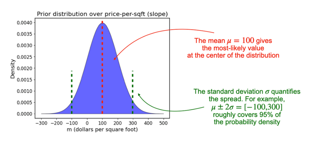
The prior distribution of the slope 𝑚 in the linear regression model, which gives the highest probability to the value 100 but there’s a high level of uncertainty in this value, quantified by the large spread of the distribution.

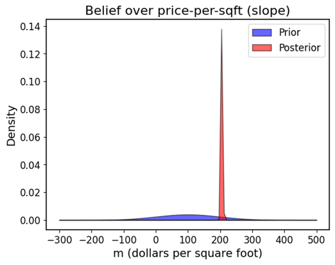
The prior and posterior distributions of the slope 𝑚. The posterior distribution sharply peaks around the true value 𝑚 = 200 to reflect the insight from the observed data.

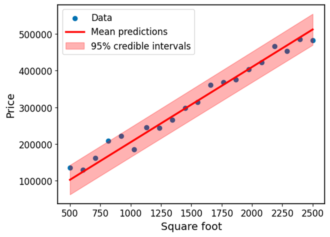
The posterior predictive distribution of individual datapoints in the test set, illustrated by the predictive mean and 95% credible intervals. Most datapoints in the training set falls within the credible intervals.

• Conjugate priors are special priors that yield posteriors in the same family of distributions, enabling closed-form Bayesian updates.
• By switching from discrete to continuous priors (such as the beta distribution for proportions), we avoid the need to round or bin parameter values.
• A beta prior combined with a binomial likelihood yields a beta posterior—this is known as the beta–binomial conjugate pair.
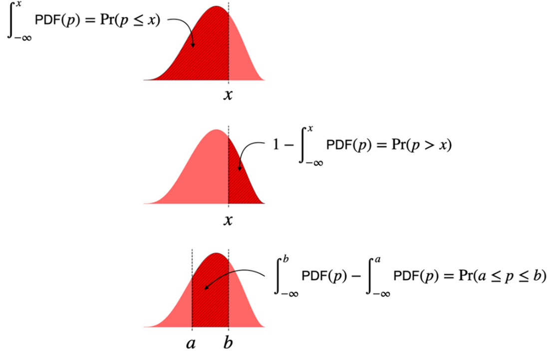
• In the continuous setting, probability densities replace probability masses, and integrals replace sums to compute probabilities.
• The beta distribution is flexible and can represent a wide range of prior beliefs using its two hyperparameters.
• Conjugate priors simplify the math of Bayesian inference by eliminating the need for complex integration in the posterior normalization.
• The normal–normal conjugate pair models real-valued parameters like the slope in linear regression, yielding a normal posterior.
• Bayesian linear regression yields not just a point estimate but a distribution over the slope, capturing uncertainty.
• The posterior predictive distribution for new datapoints includes both the uncertainty in the parameters and in the observation noise.
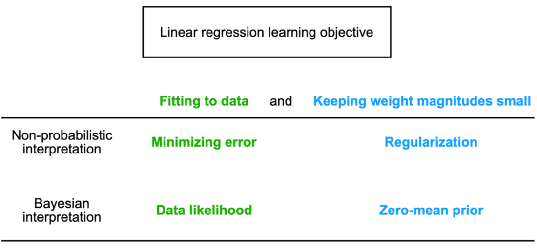
• Bayesian priors play a similar role to regularization in the traditional linear regression model, controlling model complexity especially in low-data settings.
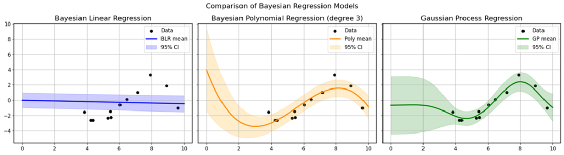
• Gaussian processes can be seen as a generalization of Bayesian linear regression to infinite-degree polynomials.

FAQ