9 The World of Statistical Modeling

This chapter presents statistical modeling as a pragmatic toolkit for explaining patterns, making inferences, and generating predictions from data. It emphasizes that a small set of model classes can power many deliverables and that “better” depends on purpose and context. Core classes include regression (continuous outcomes), classification (categorical outcomes), time series (temporal forecasts), survival analysis (time-to-event), hierarchical models (nested structures), clustering (unsupervised grouping), and dimension reduction (simplifying inputs). The problem you need to solve—and the information you can reliably collect—guides the choice of class and formulation.

The chapter outlines a disciplined workflow: select an appropriate model and formula, fit it, evaluate, and iterate. Key diagnostics span coefficients (effect estimates), model-level metrics (e.g., R-squared, adjusted R-squared, F-statistic) and comparative criteria (log-likelihood, AIC, BIC), plus residual analysis to check assumptions (linearity, normality, heteroscedasticity). Exploratory analysis and feature engineering are central—visualizing relationships, deriving informative variables, and addressing collinearity or transformations when needed. A worked example forecasting New York City rat complaints demonstrates joining data sources, creating time-based features (e.g., weekday), removing bad records, testing transformations, and balancing fit versus complexity while monitoring residuals and information criteria.

Finally, it distinguishes between explanatory and predictive deliverables and anchors both in stakeholder needs. Explanatory models clarify strength, direction, and plausible mechanisms to support strategy; predictive models focus on out-of-sample accuracy and operational utility, using train/test splits and metrics like RMSE (for regression) or precision/recall/AUC (for classification). The chapter discusses packaging predictions as batch or live outputs, deployment considerations, and the value of pairing production models with accessible explanations. Throughout, it stresses communicating assumptions and limits, iterating thoughtfully, and delivering equations, tools, or services that stakeholders can act on.

A linear regression with two variables (a predictor and outcome) is one of the simplest forms of statistical models to fit to your data.

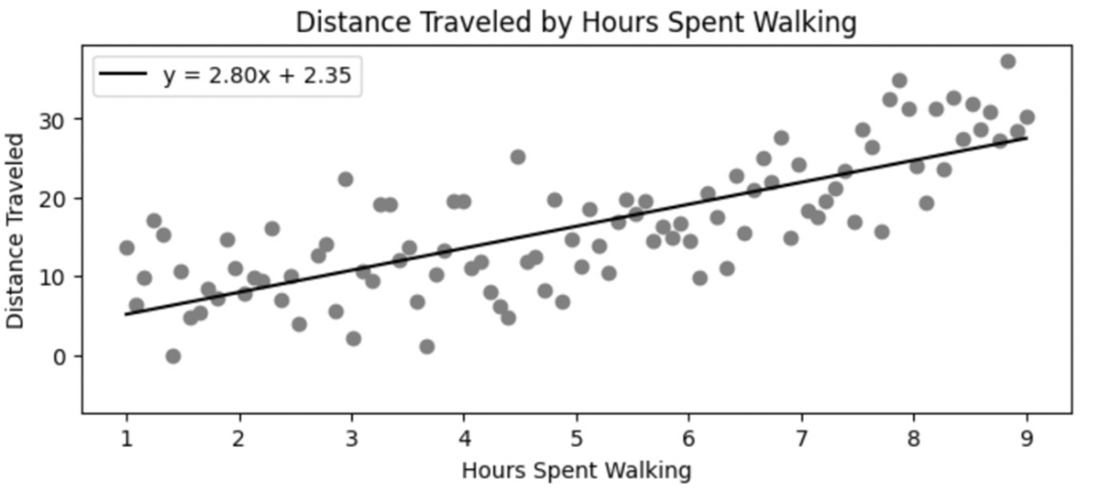
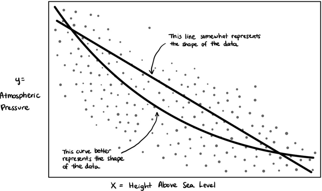
Many mathematical formulas can represent the shape of relationships in your data, such as a linear formula (line) or a polynomial (curve) formula.

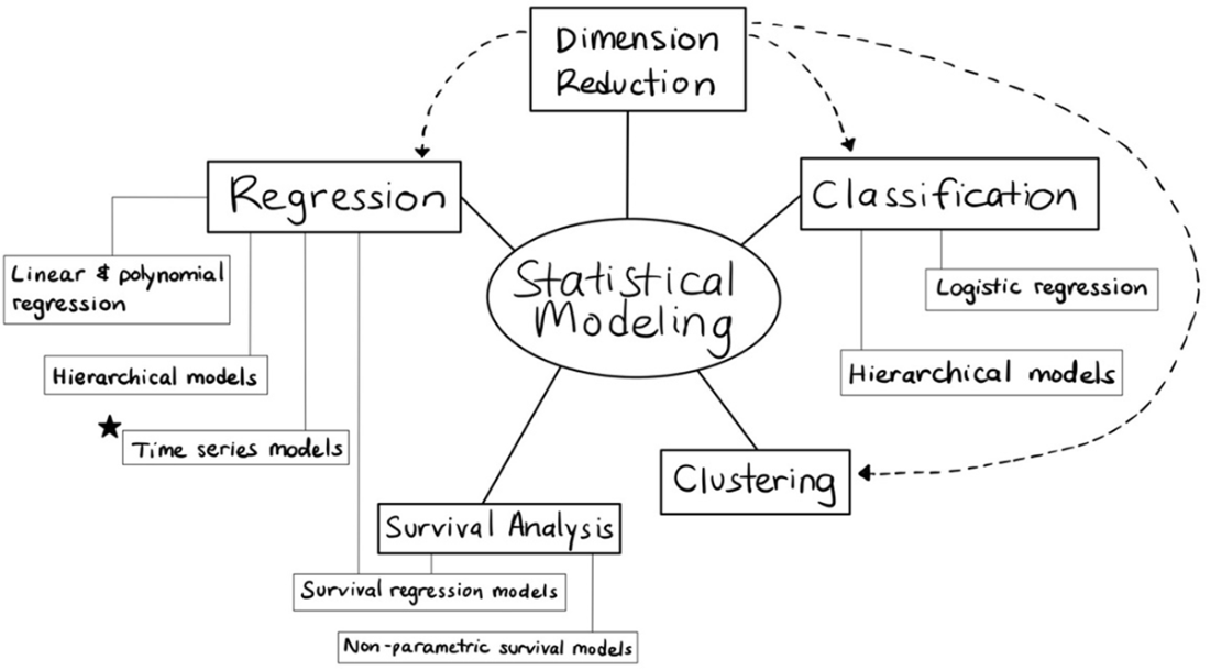
Map of common classes of statistical models organized by the problem they solve.

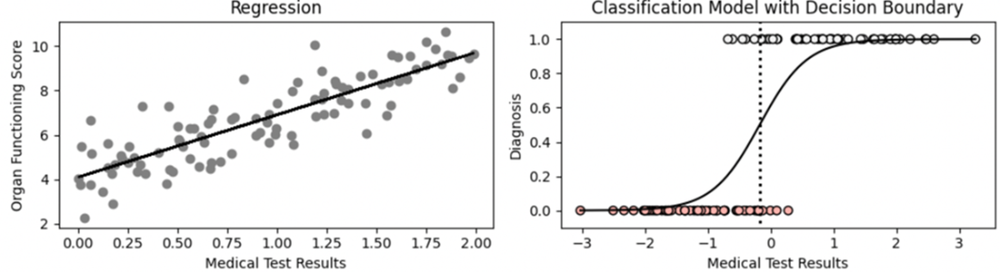
Regression and classification models are among the most commonly used in statistics.

Time series models look for patterns in data captured over time to predict future values.

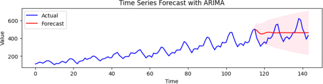
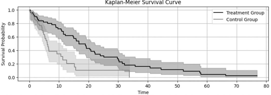
Survival analysis models predict the probability of surviving an event after each time period.

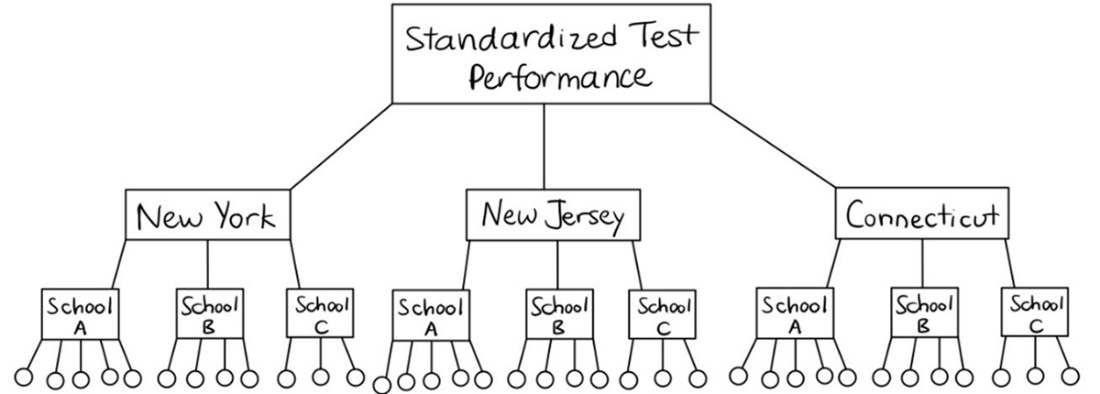
Hierarchical models allow you to capture multiple levels of underlying patterns in your data.

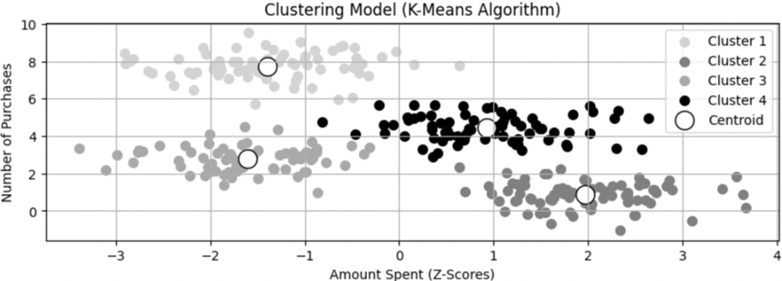
Clustering models look for underlying patterns to create categories based on the data.

Dimension reduction models are used when models contain too many inputs to tease out the effect of any individual variable.

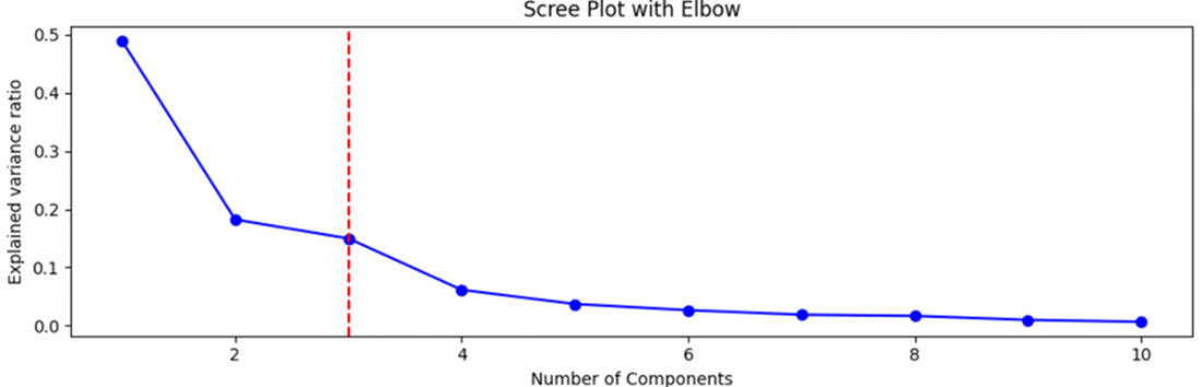
Often, a large number of variables can be represented with a fewer number of "components."

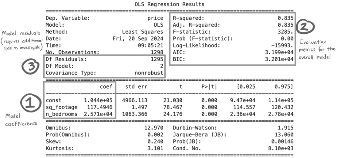
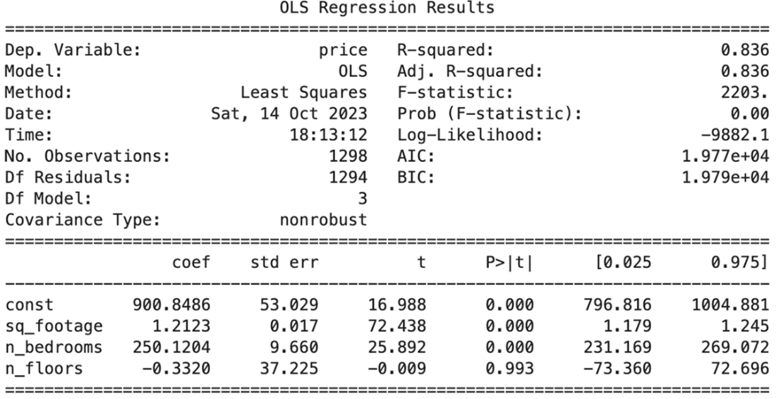
A statsmodels summary output for an ordinary least squares regression predicting housing prices using the square footage and number of bedrooms.

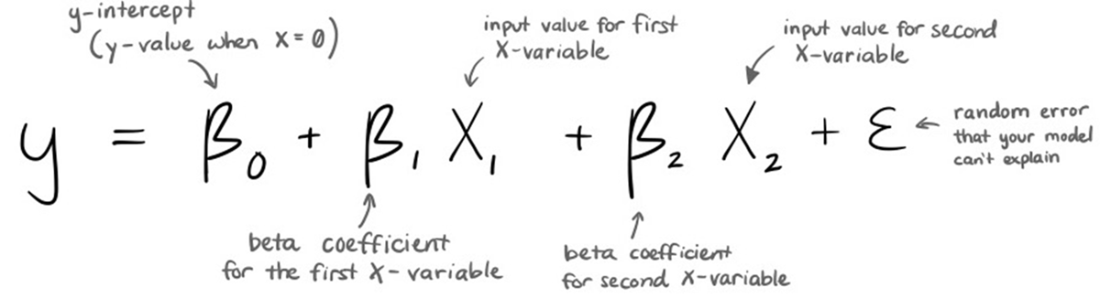
Linear multiple regression equation with two independent variables and an error term

A linear model estimating the price of a house based on the price per square foot and number of bedrooms. The carat on the y denotes that we are working with an estimate.

Estimating a house price with new inputs not included in the original sample.

Housing prices summary with an added predictor that introduces complexity to the model.

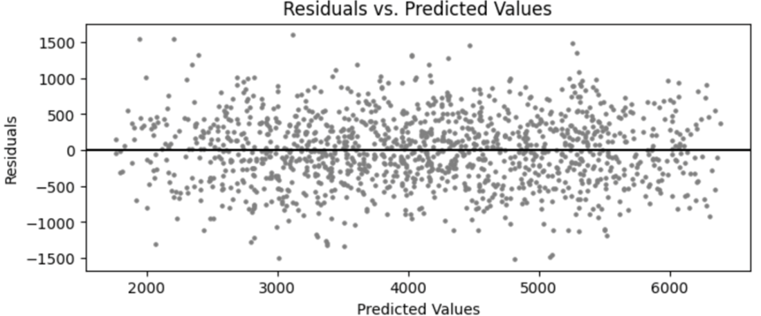
Scatterplot of residuals vs. the predicted values for each record in the dataset used to fit the regression model.

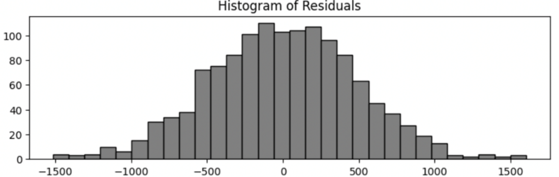
Distribution of residuals for the housing prices model.

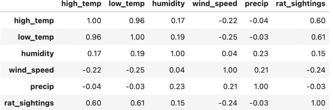
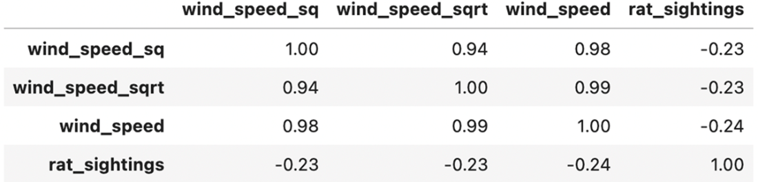
Pearson's correlations between daily weather and rat sightings, rounded to two decimal points.

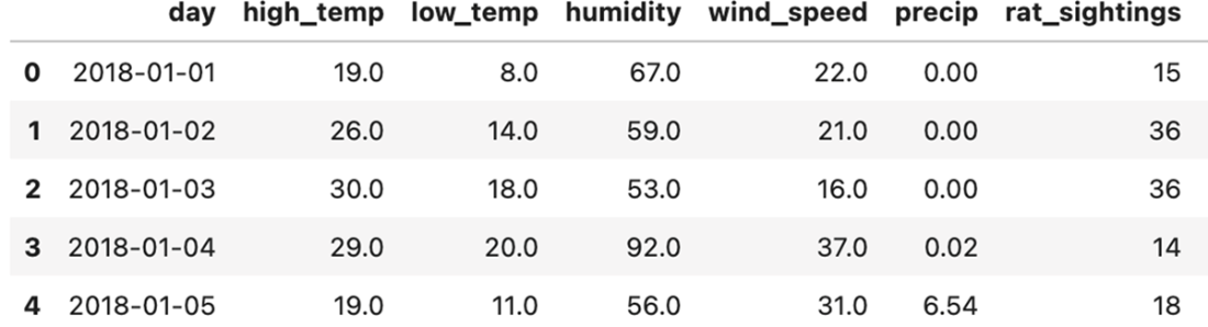
Preview of the combined rats and weather dataset

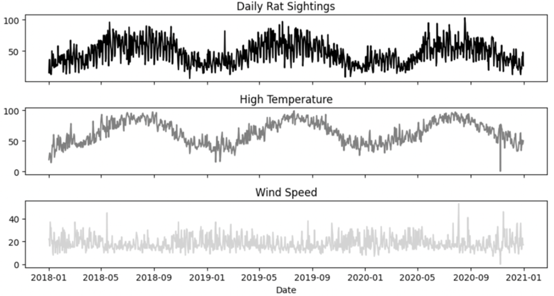
Time series plots of our outcome variable and two selected predictors.

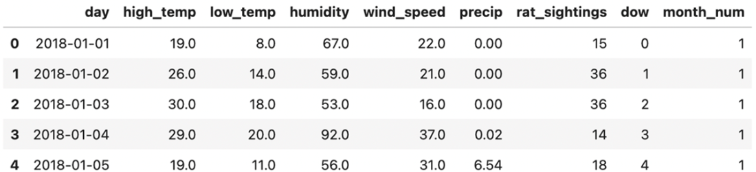
First few rows showing the new integer columns with the day of the week and month number.

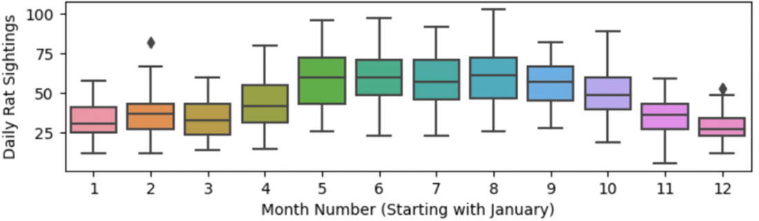
Boxplots showing the median and distributions of rat sightings for each month

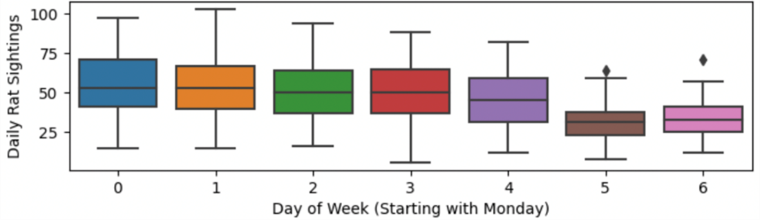
Boxplots showing the median and distributions of rat sightings for day of the week

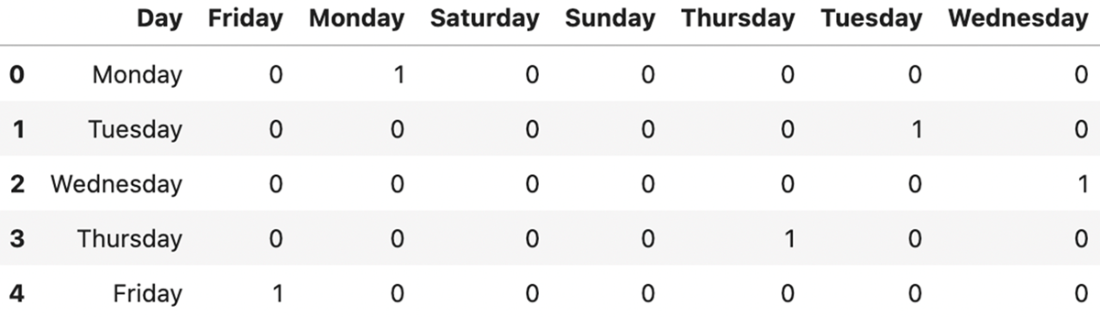
Dummy coded variables for each day of the week. The final set of variables for a model will often exclude the last category, which is implied when all other categories are absent.

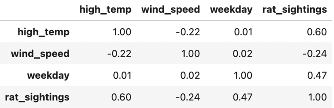
Correlation matrix including the new binary weekday column.

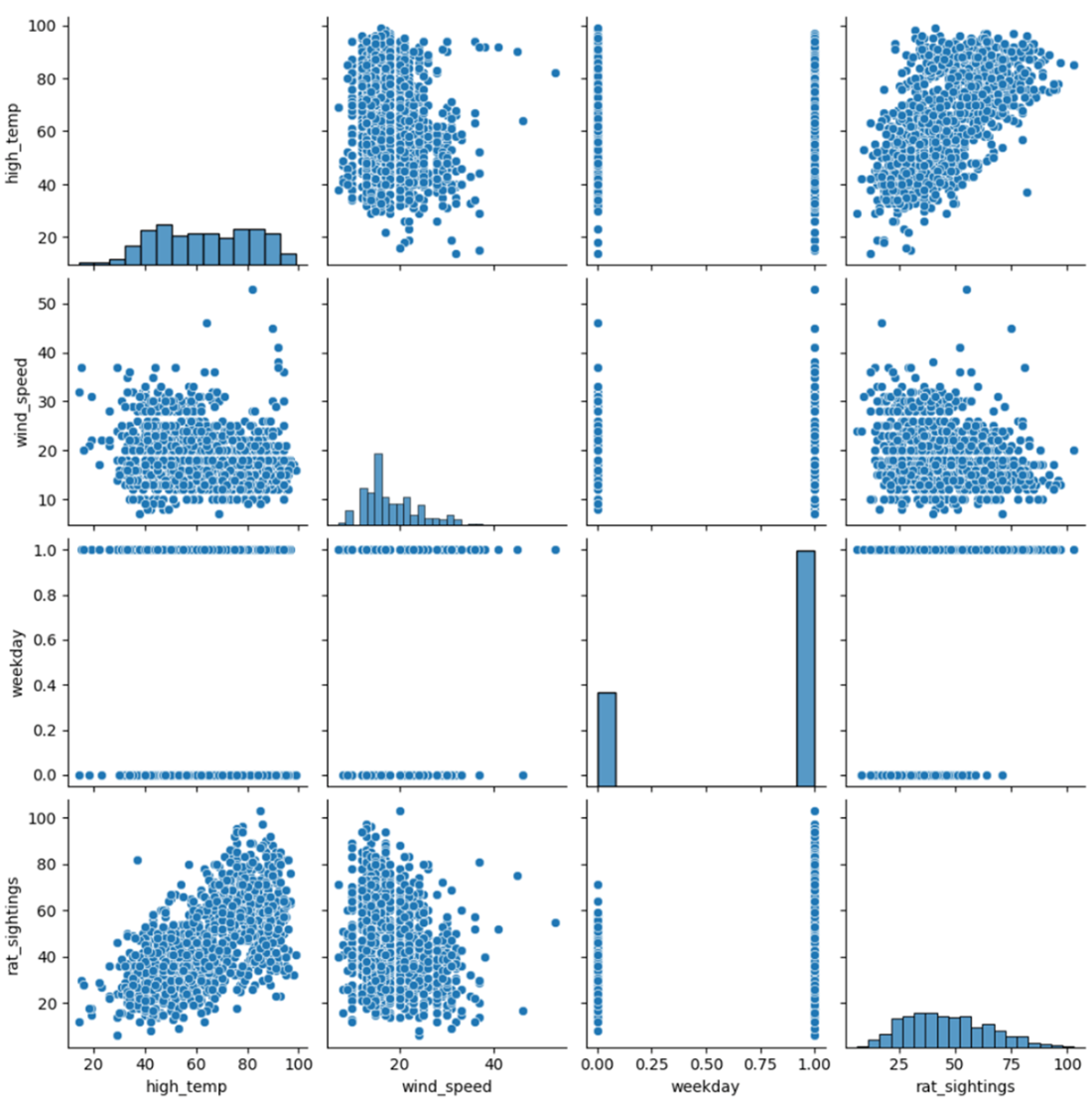
Seaborn pairplots are similar to a visual representation of a correlation matrix.

Pearson's correlation values between the transformed variables and the outcome

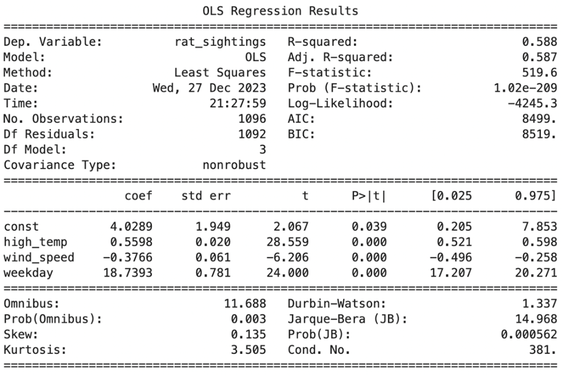
Summary of a linear regression model predicting daily rat sightings.

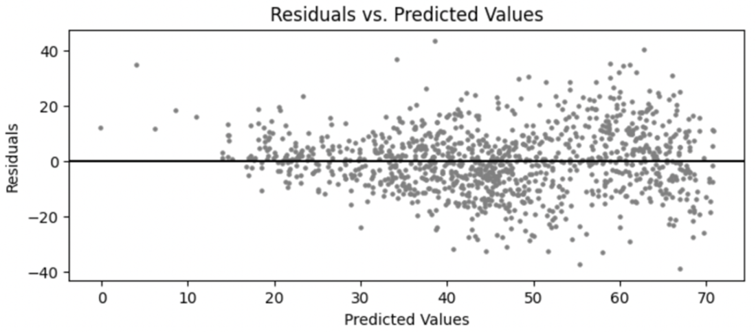
Plot of residuals against the predicted rat sighting values

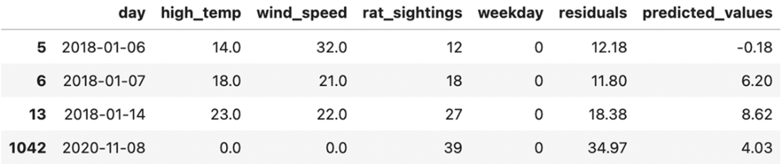
Preview of dataset records with low predicted values

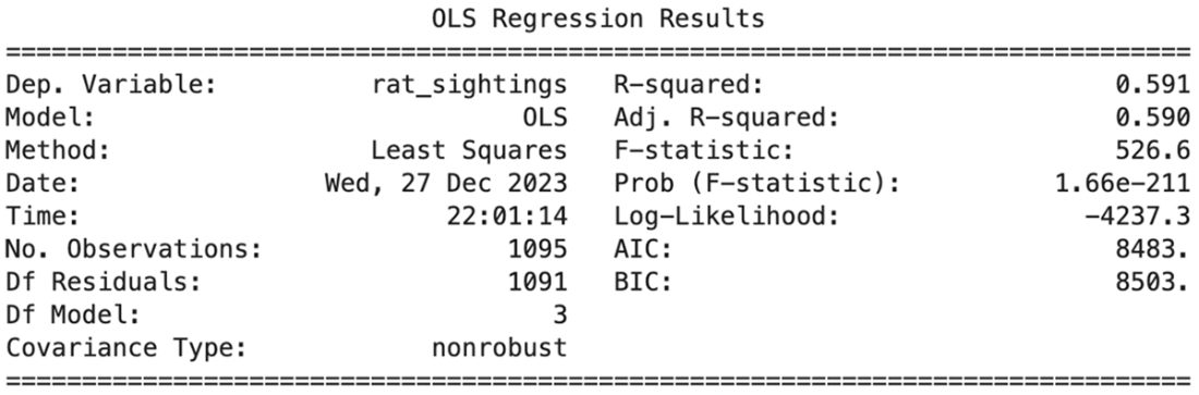
Overall regression results for the model with bad data removed.

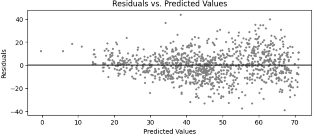
Residual plot for an adjusted model, showing the removal of the outlier

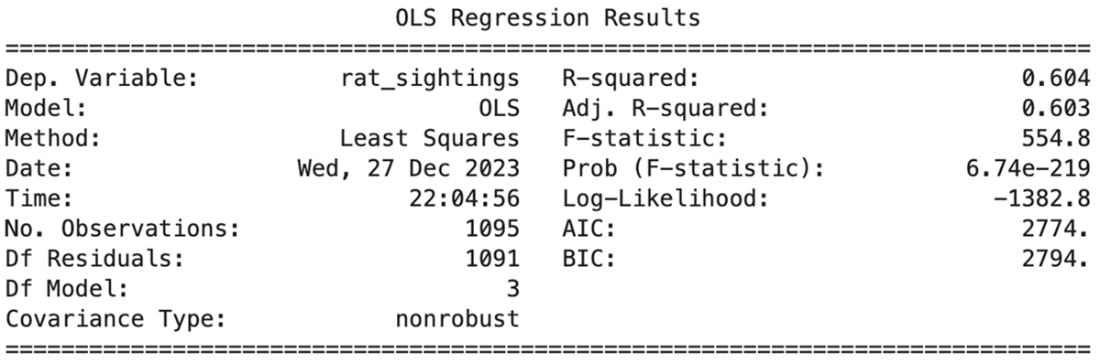
Overall regression results for the model with a transformed y-variable.

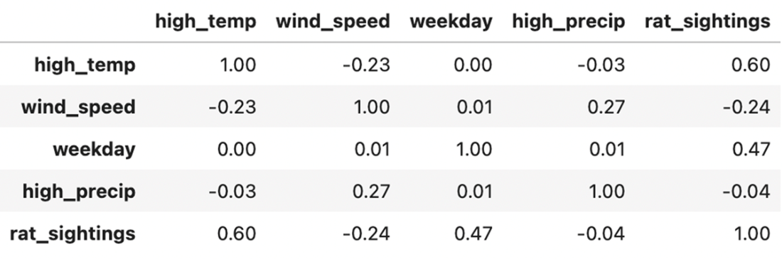
Correlation matrix including the new column for high vs. low precipitation.

Regression results with the added high precipitation variable.

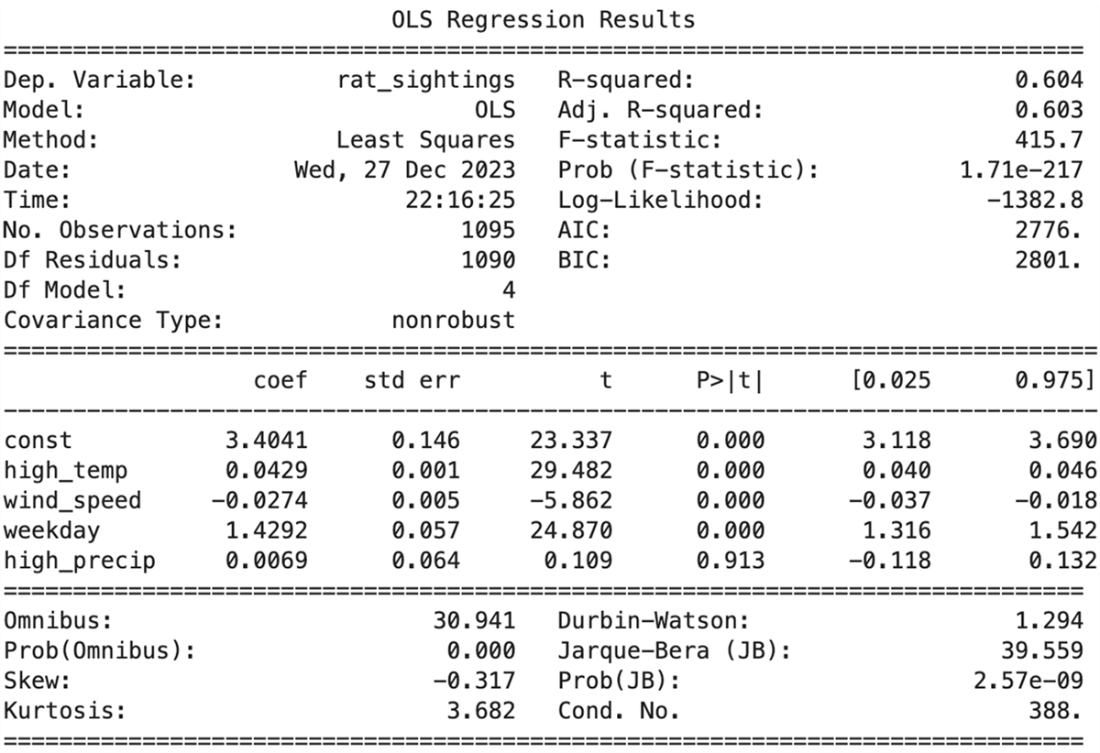
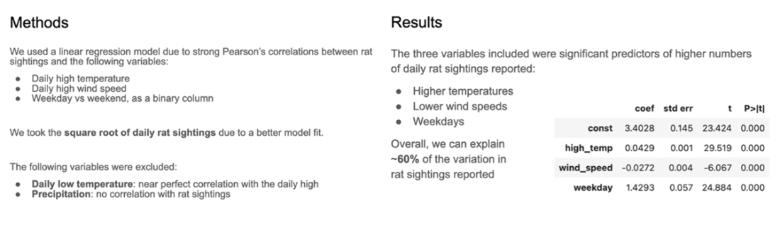
Slides showing the summary of methods & results that document conclusions about individual input variables.

• There are many classes of statistical models available tailored to solving specific types of problems:
• Regression models use one or more predictors to predict a continuous outcome (e.g., price).
• Classification models use one or more predictors to predict a categorical outcome (e.g., purchased or not purchased).
• Time series models use historical data collected over time to forecast values for future time periods.
• Survival analysis is similar to regression modeling, where the outcome variable of interest is whether a participant or data point "survives" past a specific time period. These models are often used in clinical settings to understand the probability of surviving an illness for certain periods of time.
• Hierarchical models account for the nested structure of your data, such as when participants belong to one or more hierarchical groups (e.g., a classroom, a school, a district) that may impact your outcome.
• Clustering models identify underlying patterns in your data without an outcome variable (unsupervised learning in machine learning). These algorithms can help identify groups of individuals or data points that were not discoverable by visual observation alone.
• Dimension reduction techniques consolidate large sets of predictor variables into a smaller set of components. Each component represents a significant pattern or aspect of variation within the original data, thus simplifying the dataset while retaining its most informative features.
• Model evaluation metrics are available for each class of models, giving us information we can use to diagnose the quality of its fit to the data. When working with regression models, we can use the following metrics to evaluate a model:
• R-squared (R²) represents the proportion of variance in your outcome variable explained by all of your input variables.
• Adjusted R² adjusts the original value, penalizing the score for each additional variable you include in your model. This score enables you to balance model quality and complexity.
• The F-statistic tests the overall significance of the model.
• The log-likelihood is one of several relative metrics that tell you how well your model fits the data. These can be used to compare the relative quality between multiple model iterations.
• AIC and BIC are relative metrics used to evaluate a model's overall quality. Each score penalizes model complexity, enabling you to balance the fit and complexity to select a best-fit model.
• Residuals are the differences between the observed and predicted outcome values that help you understand the parts of your model not explained by your predictors. When residuals show patterns that aren't normally distributed, it hints at issues such as missing transformations or variables.
• Statistical modeling systematically involves data preparation, analysis, and iterative refinement. It begins with understanding your problem, gathering & cleaning data, and fitting one or more models to best represent that data.
• Exploratory analysis is a crucial initial step that involves examining data through visualizations and summary statistics to identify patterns and spot anomalies, setting the stage for informed model building.
• Feature derivation or feature engineering involves creating new variables from your existing dataset to better represent the underlying processes in your model. This can include transformations (e.g., square root), extracting components of a column (e.g., month number in a date), or creating combinations of multiple variables (e.g., combined profit).
• Evaluating assumptions involves verifying the validity of foundational assumptions inherent to your chosen model. This can include checking linearity, normality, homoscedasticity, and the independence of residuals. These steps are necessary to ensure your model's reliability.
• Models are refined using absolute and relative indicators to adjust variables, tune parameters, or change the modeling approach.
• Explanatory and predictive models are two overarching categories of model deliverables that guide your model fitting and optimization strategy.
• Explanatory models showcase the relationships between individual variables and an outcome, emphasizing interpretability and the statistical significance of coefficients. The predictors included in your model are guided by domain knowledge and rigorously evaluate existing theories and hypotheses. Explanatory model deliverables are usually prepared as detailed reports with recommendations for the intended audience or stakeholder.
• Predictive models focus on the accuracy of out-of-sample predictions and generalizability to new data. Predictions can be delivered in many formats, including interactive tools using the model's equation, batch predictions on large datasets, or live predictions that influence actions taken in real-time.

FAQ