5 The Statistics You (Probably) Didn’t Learn: Non-Parametric Tests, Chi-Square Tests, and Responsible Interpretation
This chapter broadens the analyst’s toolkit beyond familiar parametric tests by explaining when and why non-parametric and chi-square methods are better choices, and how to interpret them responsibly. It situates parametric statistics historically and critically—highlighting their early 20th-century origins, assumptions (notably normality and variance homogeneity), and overuse—then argues for method choices that fit real data, which are often non-normal, ordinal, categorical, or drawn from very large samples. The emphasis is on asking the right questions, matching them to flexible methods, and communicating results with clarity about what was actually compared.
The chapter surveys practical non-parametric alternatives: Mann-Whitney U for two independent groups, Wilcoxon signed-rank for paired data, Kruskal-Wallis for two or more independent groups (with Dunn’s post hoc), and Friedman for three or more related groups (with Wilcoxon post hocs and Bonferroni correction). These rank-based tests are distribution-agnostic, work with continuous and ordinal data, and are robust to unequal variances, but they compare medians/ranks rather than means, can lose power when parametric assumptions hold, are sensitive at extreme sample sizes, and require care with tied ranks. The guidance stresses reporting medians, using appropriate post hocs, and—when feasible—validating conclusions by running both parametric and non-parametric tests to see whether inferences converge.
For categorical questions, the chi-square family is presented as a versatile way to compare observed versus expected frequencies: goodness-of-fit (one variable), independence (two variables in contingency tables), and trend tests. Chi-square thrives with larger samples but needs adequate expected counts and often follow-up pairwise comparisons to locate disproportionality. The chapter closes with responsible interpretation: understanding Type 1 and Type 2 errors, planning sample sizes and alpha levels thoughtfully, checking assumptions, using replication or bootstrapping where possible, and controlling confounding via study design, stratification, and covariate-aware models. It firmly warns against p-hacking—iterating tests, variables, designs, or selective data edits until significance appears—and advocates transparent, domain-informed communication about what was tested and what the results truly mean.
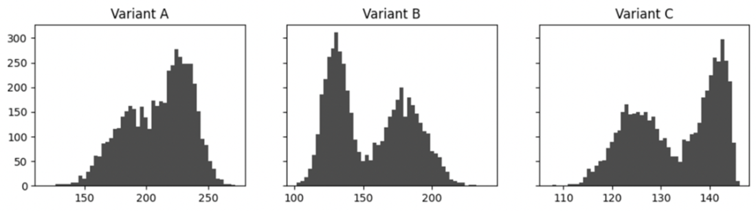
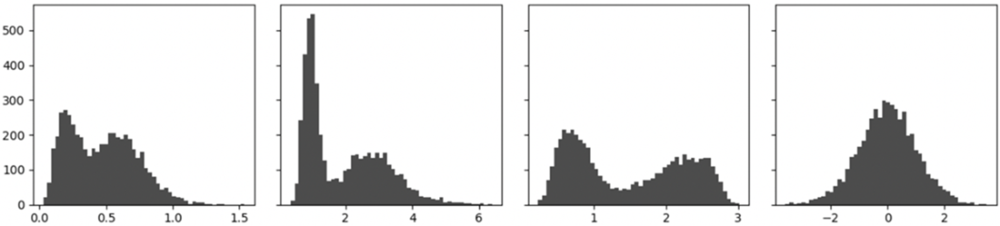
The distribution of each group shown is bimodal, which traditional measures of central tendency won’t be able to detect.
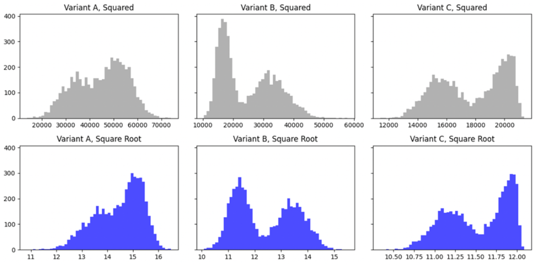
Square and square root transformations of the original bimodal distributions.
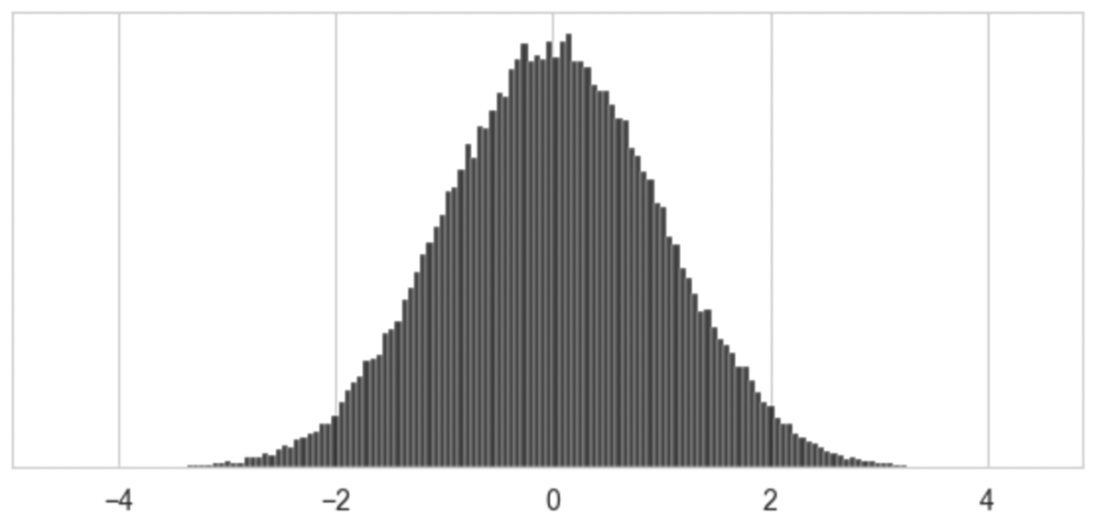
The bell curve/normal curve is ever present in statistics and does occur naturally for a handful of phenomena, such as the distribution of human heights.
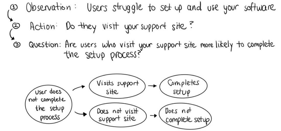
Visual Representation of a Causal Phenomenon with Observation-Oriented Modeling
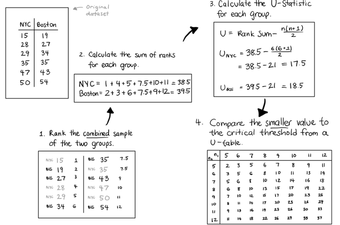
Steps to calculating the U-statistic
The Mann-Whitney U test can be leveraged for any distribution shapes displayed, whereas the t-test is only appropriate for the final (normal) distribution shape.
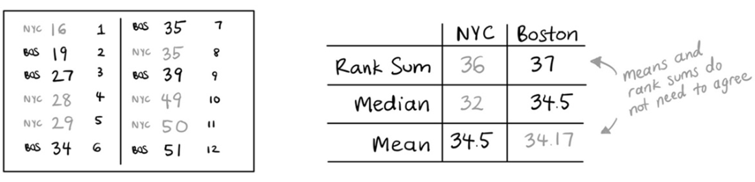
U-values or rank sums agree directionally with the median of a dataset but don’t always align with the interpretation of the mean. Be careful in conflating your interpretations!
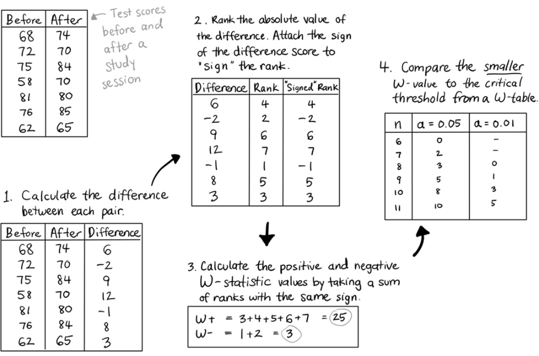
Steps to calculating the W-statistic
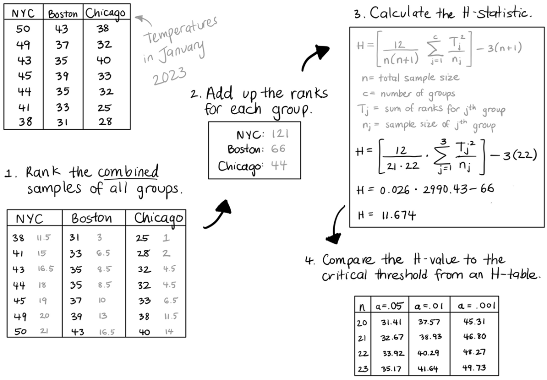
Steps to calculating the H-statistic with 3 groups and n=21
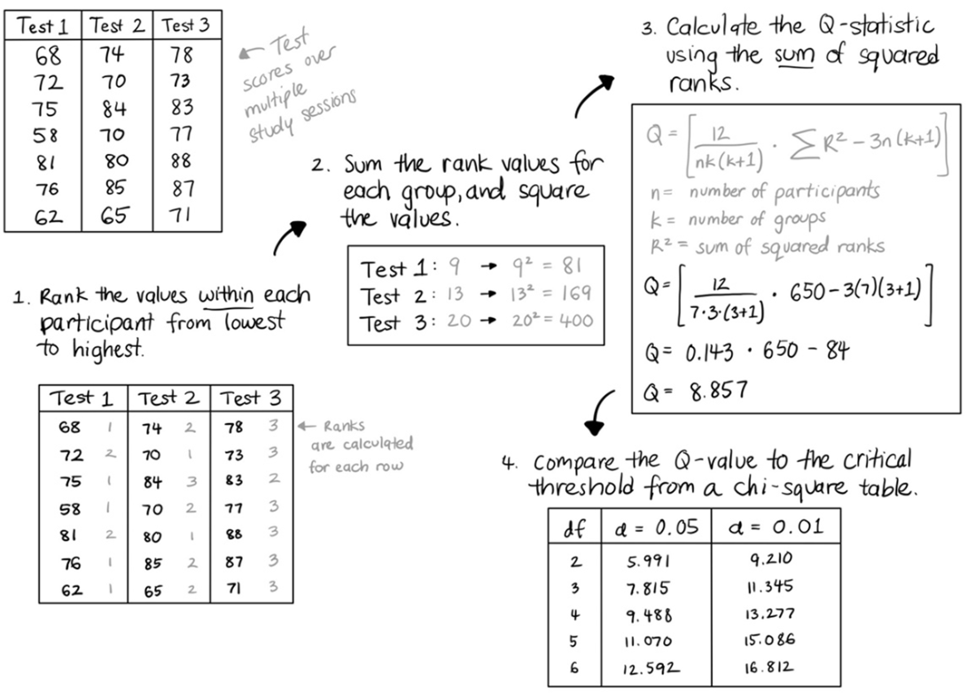
Steps to calculating the Q-statistic
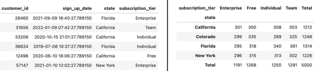
Comparisons of two categorical variables can be presented as a contingency table, pivoting the results into summarized rows and columns you can easily view.
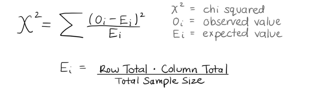
Breakdown of the equation for the X2 (chi-squared) test
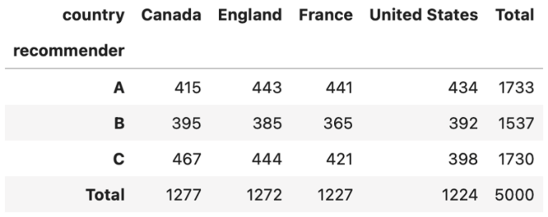
Count of users who engaged with the feature broken out by country and experiment group.
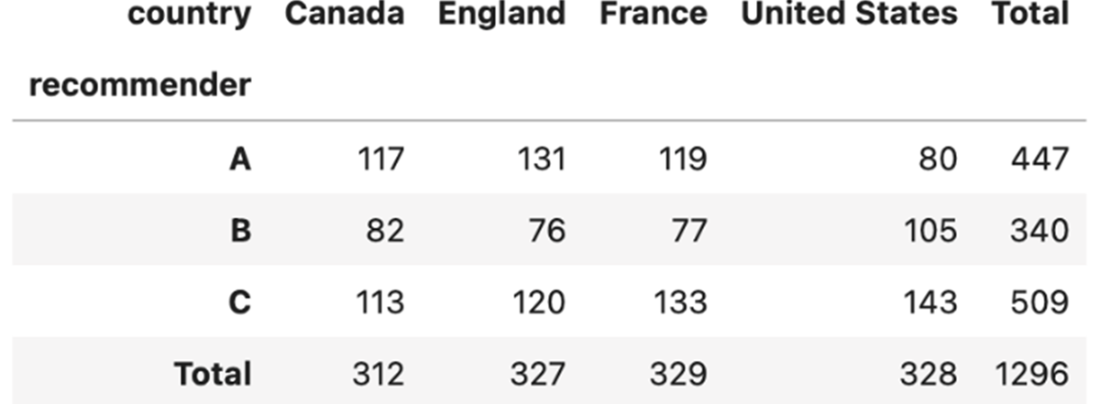
Summary table of the number of recommendation clicks by group.
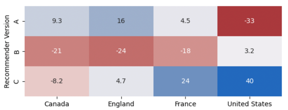
Human-readable heatmap of differences between observed and expected click rates.
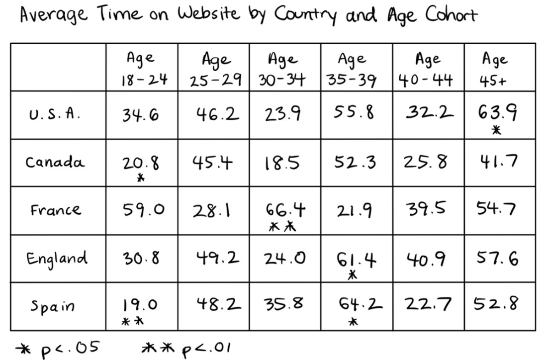
Your author implores you not to run excessive multiple comparisons, even with a sufficiently large sample size.
The majority (but not all) of bootstrapped samples have t-values above the absolute value of the critical threshold
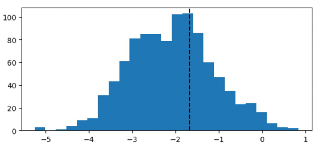
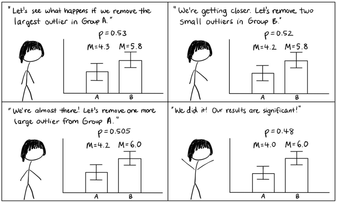
P-hacking involves testing a dataset indefinitely until something returns a significant value.
Summary
- The majority of parametric statistical tests were developed 100 years ago or more for specific types of analysis and have since become the dominant method of choice for most fields of study and work. However, these tests are not ubiquitous and are not always the best choice for every analysis.
- Non-parametric statistical tests are alternatives to parametric statistical tests that do not make assumptions about the underlying distribution of the data. They can be used with a broader variety of data types than parametric statistical tests (you can use either continuous or ordinal data), providing analysts with a wide range of options.
- There is a wide range of non-parametric tests for group comparisons. Each test compares the ranks and relative positions of the data points in each group rather than making calculations based on the actual values of the data points. The most common are:
- The Mann-Whitney U test for comparing two independent samples
- The Wilcoxon Signed-Rank test for two dependent samples
- The Kruskal-Wallis test for two or more independent samples
- The Friedman test for three or more dependent samples
- Post-hoc tests are statistical comparisons conducted after a test with three or more groups indicates significant differences among group means, used to identify which specific groups differ from each other. These tests apply corrections to control the increased risk of false positives (Type 1 errors) that occur due to multiple comparisons, ensuring the reliability of the results.
- The chi-square test is a common test that you can use to compare one or two categorical variables. The test compares the difference between the observed to expected frequencies for each row and column in a contingency table.
- A Type I error occurs when a true null hypothesis is incorrectly rejected, representing a false positive in hypothesis testing. Conversely, a Type II error happens when a false null hypothesis is mistakenly accepted as true, resulting in a false negative.
- Part of being a responsible analyst involves ensuring the integrity of your approaches, even when your stakeholders aren’t watching. Choose your design ahead of time, and don’t be afraid to report non-significant results for the long-term accuracy of your work and the trust of your stakeholders.
FAQ
When should I choose non-parametric tests, and what trade-offs should I expect?
Use non-parametric tests when your data violates parametric assumptions (non-normality, unequal variances), the distribution is unknown/bimodal, or your measures are ordinal. They are robust to shape assumptions and often work well with ranks/medians. Trade-offs: they typically have lower power than parametric tests when assumptions are met, compare medians/ranks (not means/variances), and may be sensitive at very small or very large sample sizes. Plan for post-hoc tools that may require extra packages.
What are the non-parametric alternatives to common parametric tests?
- Independent samples t-test → Mann-Whitney U (Wilcoxon rank-sum)
- Paired/repeated t-test → Wilcoxon signed-rank
- One-way ANOVA (between-subjects) → Kruskal-Wallis (with Dunn’s post-hoc)
- One-way repeated measures ANOVA → Friedman (pairwise Wilcoxon post-hocs with Bonferroni)
- Categorical comparisons → Chi-square tests (goodness-of-fit, independence, trend)
How does the Mann-Whitney U test work, and what should I watch out for?
It compares medians between two independent groups using rank sums and the U-statistic; significance is based on the lower U relative to a critical value. Advantages: robust to non-normality and unequal variances; works with ordinal data. Watch outs:
- Small samples can inflate false positives.
- Large samples can increase false negatives for this test.
- Many tied ranks reduce power; minimize ties where possible.
- No sign to indicate direction—use group medians or rank sums for direction.
- Report medians, not means; rank-based results align with medians.
When should I use the Wilcoxon signed-rank test, and what assumptions matter?
Use it for two related/repeated measures when normality is violated. It ranks absolute pairwise differences, applies signs, and compares summed positive vs negative ranks (W-statistic). Key assumptions:
- Paired differences should be roughly symmetric around the median (check visually/skewness/kurtosis).
- Reduce ties in differences (e.g., jitter small decimals) to maintain power.
Report medians and helpful proportions (e.g., percent improved) alongside the test.
How does the Kruskal-Wallis test compare to ANOVA, and how do I run post-hoc tests?
Kruskal-Wallis compares medians across 2+ independent groups using ranked data (H-statistic). It does not indicate direction; use post-hocs to locate differences. Notes:
- H reflects magnitude, not direction; inspect group medians/ranks for direction.
- Use Dunn’s test with a Bonferroni-type correction for multiple comparisons.
- With exactly two groups, KW and Mann-Whitney yield nearly identical p-values.
What is the Friedman test and how do I interpret and follow it up?
Friedman compares 3+ related samples (repeated measures) using summed squared ranks (Q, often treated as chi-square). Unlike U/W tests, significance requires Q greater than the chi-square critical value. If significant, run pairwise Wilcoxon-based post-hocs with a Bonferroni correction to identify which time points/conditions differ.
What is a chi-square test, and when should I use each type?
- Goodness-of-fit: does one categorical variable’s observed distribution match expected proportions?
- Test of independence: are two categorical variables associated (contingency table)?
- Test for trend: is there an ordered pattern across categories (e.g., over time)?
Chi-square compares observed vs expected frequencies; large samples increase sensitivity (small differences become detectable).
What are key considerations and pitfalls when running chi-square tests?
- Ensure expected frequency ≥ 5 in each cell; combine sparse categories if needed.
- Stratify/randomize thoughtfully; validate balanced assignment before outcome tests.
- Inspect where disproportionality occurs: subtract expected from observed and visualize (e.g., heatmap).
- Use pairwise 2x2 post-hoc comparisons with multiple-comparison corrections to locate differences.
How can I reduce false positives and false negatives in practice?
- Pick appropriate tests and check assumptions; transform data if suitable.
- Set conservative alpha (≤ 0.05, or 0.01 when stakes are high) and interpret p-values contextually.
- Limit multiple comparisons; use corrections for post-hocs.
- Plan adequate sample size (a priori power analysis) to avoid underpowered tests.
- Replicate or bootstrap to assess result stability.
- Account for confounders via design (stratification, randomization) and modeling (covariates, ANCOVA, regression).
What is p-hacking, and how do I avoid it?
P-hacking is manipulating analyses (trying many tests/designs/filters until p < alpha) to manufacture significance. Avoid by:
- Pre-registering or documenting hypotheses, variables, and analysis plans.
- Avoiding post-hoc variable/design switching for inferential tests.
- Not manually removing outliers or cherry-picking subsamples/subgroups.
- Reporting all tests run, applying multiple-comparison corrections, and emphasizing effect sizes and robustness checks.
How should I communicate non-parametric results to stakeholders?
- Emphasize medians, ranks, and distribution visuals (e.g., boxplots), not means.
- State limitations (e.g., ties, sample size sensitivity, lower power).
- When possible, present converging evidence from both parametric and non-parametric tests and explain any divergence.

 Effective Data Analysis ebook for free
