4 The Statistics You (Probably) Learned: T-Tests, ANOVAs, and Correlations
This chapter grounds common inferential tools in clear descriptive logic, showing how summary statistics set the stage for rigorous analysis. It contrasts raw variation with simplified views, explaining how measures of central tendency (mean, median, mode) and variability (range, IQR, standard deviation, standard error) highlight different facets of a distribution and rely on assumptions such as normality, centrality, and symmetry. The text emphasizes diagnosing distribution shape, sensitivity to outliers and skew, and the communication pitfalls of familiar visuals like bar charts with error bars. It offers practical guidance on when to report each measure, how to pair metrics with visualizations, and why context and stakeholder-friendly explanations are essential before moving to inference.
Building on that foundation, the chapter details the logic and limits of parametric tests used everywhere—t‑tests, ANOVAs, correlations, and regressions—underscoring their strict assumptions: approximate normality (or transformability), independence, homogeneity of variance, and absence of extreme outliers. It clarifies how test coefficients, degrees of freedom, alpha levels, and p‑values work together, and why large samples can produce statistically significant but practically trivial results. To guard against spurious findings, it recommends pre‑registered thresholds, effect sizes (e.g., Cohen’s d), power analysis for minimum sample sizes, Welch variants when variances are unequal, and non‑parametric alternatives when assumptions fail—alongside strong cautions against p‑hacking and overly rigid p‑value thinking.
The chapter closes by sharpening correlation and regression practice and reporting. It distinguishes among correlation coefficients (Pearson for linear continuous data; Spearman and Kendall for ordinal or non‑linear relationships; point‑biserial for binary–continuous pairs), stresses checking linearity and using transformations when needed, and reviews regression assumptions (linearity, multivariate normality, low multicollinearity, homoscedastic residuals). Guidance focuses on stakeholder interpretation: visualize relationships, separate prediction from causation, highlight effect sizes and uncertainty, and explicitly state what the results can and cannot support. Throughout, a pharmaceutical case study demonstrates how to vet assumptions, choose tests, set conservative thresholds with large samples, and communicate accurate, actionable conclusions.
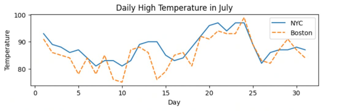
Comparison of temperatures in July between New York City and Boston.
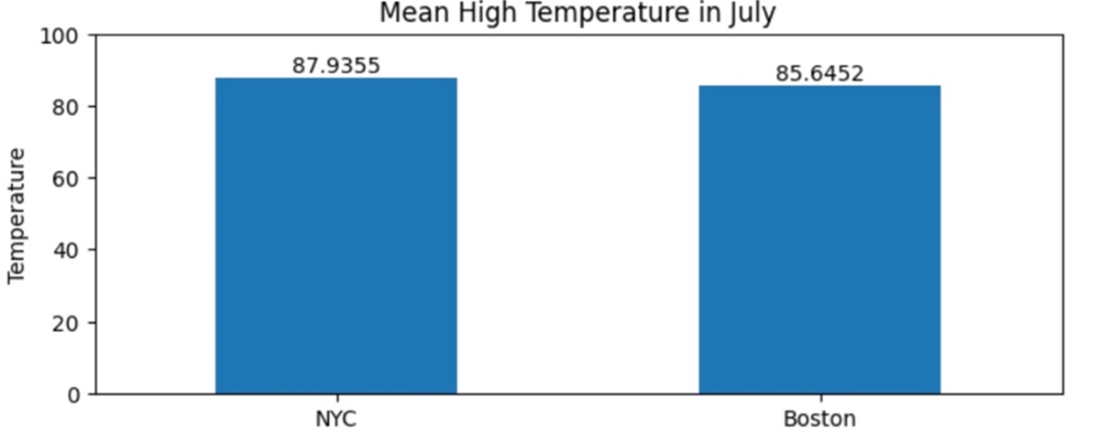
Comparison of the mean daily temperature between New York City and Boston
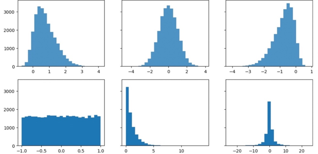
The shape of a distribution can vary widely, and different summary statistics will give you clues about those shapes.
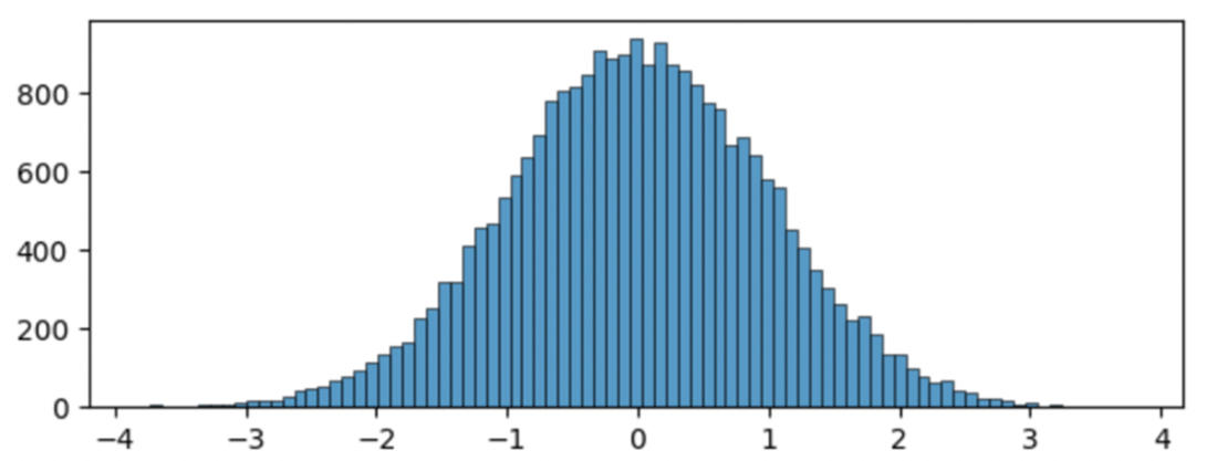
A standard normal distribution with a mean of 0 and standard deviation of 1
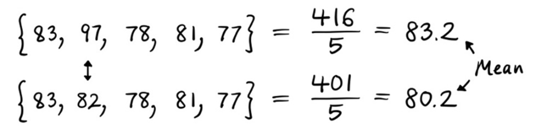
A mean calculation is highly sensitive to skewed data and outliers. The mean noticeably decreases when the highest outlier value of 97 is replaced with a value closer to the rest of the set.
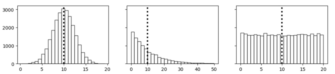
Three distinct distributions with an identical mean of 10. The interpretation of the mean or “average” is very different for each distribution.
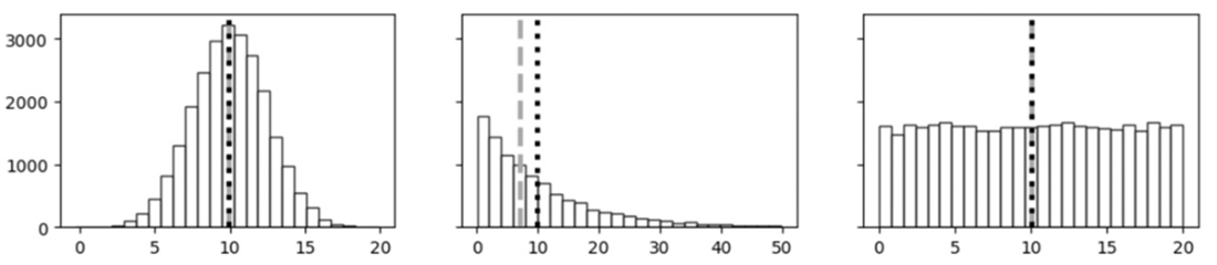
The median is robust to skewed data and outliers. When the highest outlier value of 97 is replaced with a value closer to the rest of the set, the median remains the same.

The mean (black dotted line) and median (gray dashed line) are approximately identical in the first and third distributions. The measures noticeably deviate in the second skewed distribution.
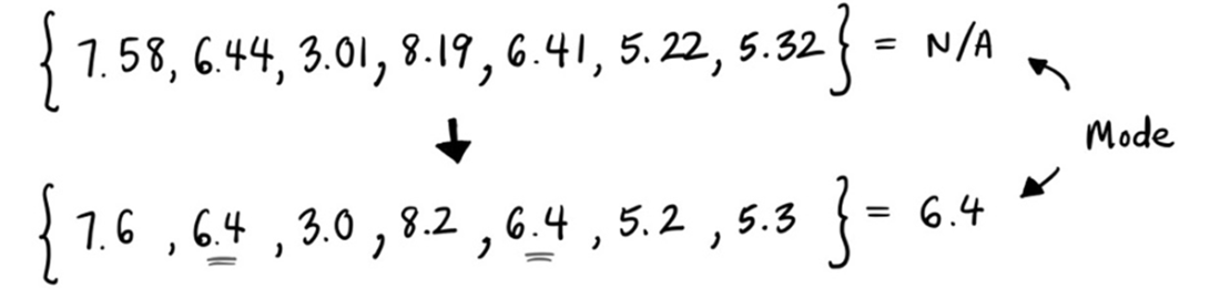
The mode is the most frequently occurring value in a dataset.
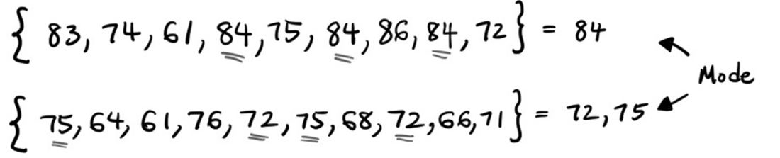
Rounding floating-point values can better showcase the mode.
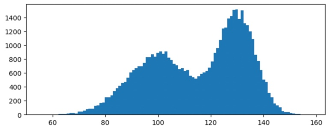
A bimodal distribution that has two modes around 100 and 130 that are best discovered by visual observation.
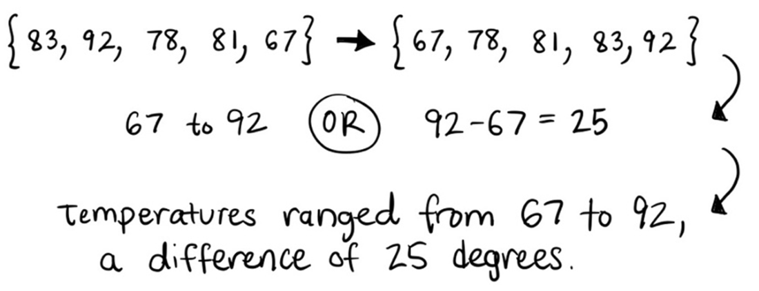
The range depicts the entire width of the dataset.
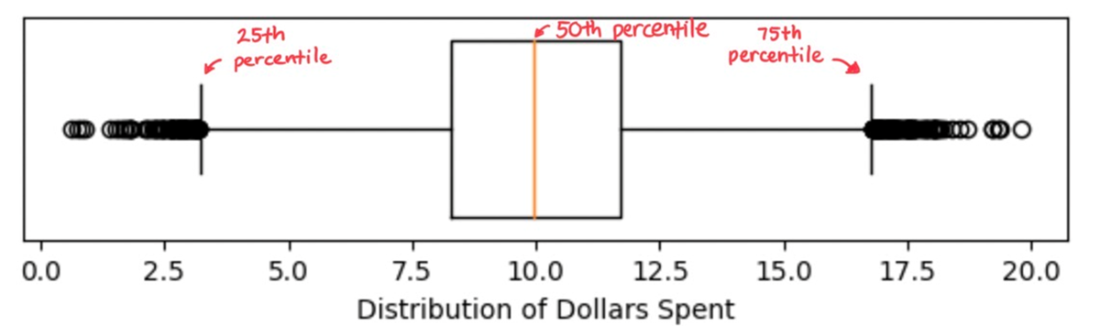
A boxplot shows the median and interquartile ranges in the box and the 5th/95th percentiles in the whiskers by default. Values outside of the whiskers are typically treated as outliers.
The standard deviation essentially takes an average of the differences from the mean.

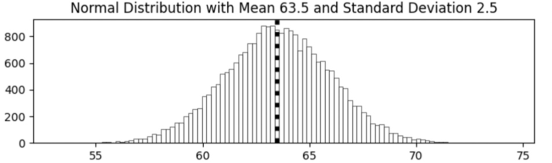
A normal distribution of heights (in inches) for men in the United States is easily generated if the mean and standard deviation are known.
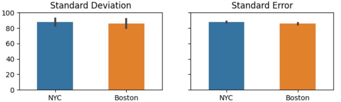
Deriving the standard deviation and standard error from the initial variance calculation.

Bar graphs with error bars are very common visualizations but run the risk of misrepresenting the underlying data and creating confusion with stakeholders around the type and purpose of the error bars.
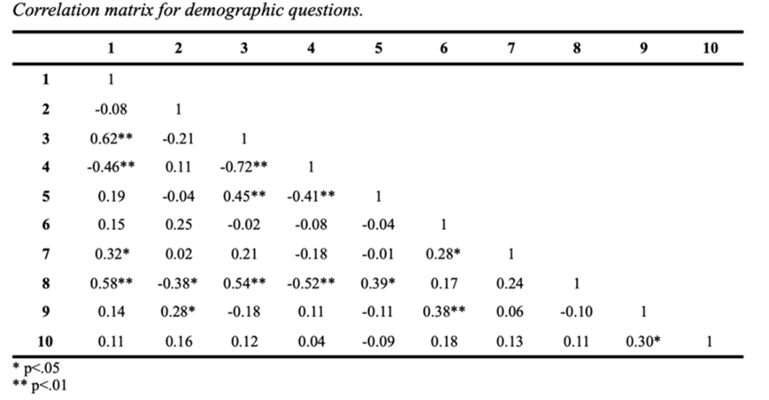
Statistical comparisons like correlations, t-tests, ANOVAs, and others are used everywhere. The example above is a correlation matrix from a program evaluation I delivered to a non-profit in 2015.
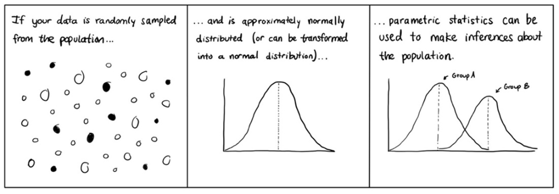
Parametric statistics assume that the population data follows a specific probability distribution and that you can make inferences about the parameters of that distribution based on your sample data.
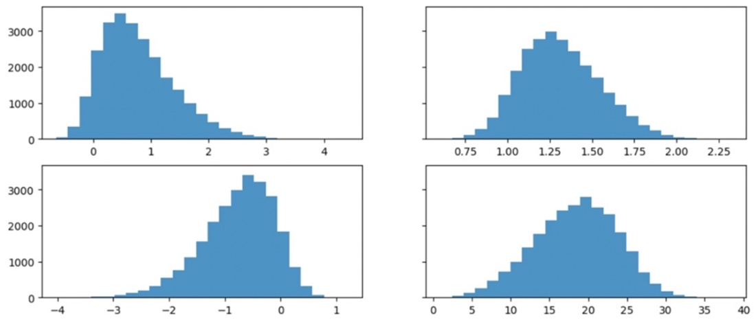
Skewed data can often be transformed into an approximately normal distribution.
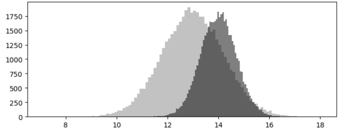
Parametric statistics generally assume that your samples have equal variances. In this example, the unequal variance leads to greater overlap between the two distributions.
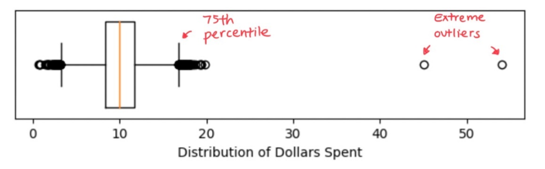
Extreme outliers are often easily detected by generating a boxplot or a histogram of your data.
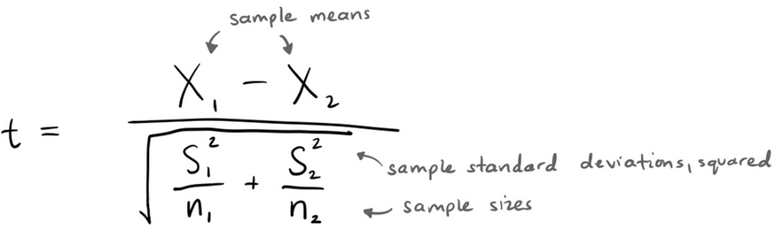
Formula for an independent samples t-test
The two groups have a non-significant difference.

The two groups still have a non-significant difference, but the t-value is larger.

Increasing the sample size by a factor of 10 yields a statistically significant result.

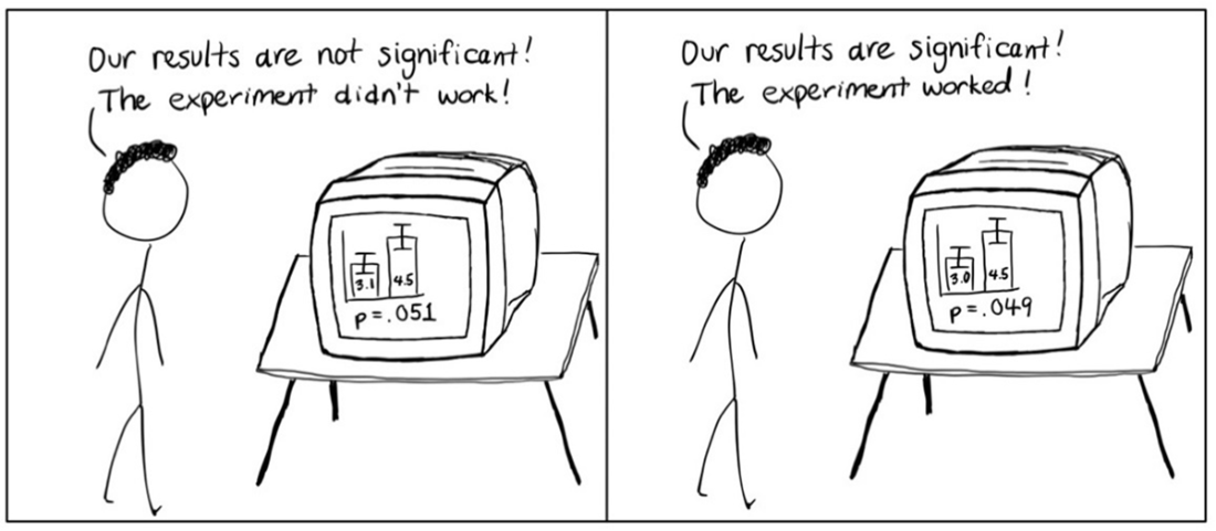
The p-value is often treated as a magical boundary that unlocks findings considered worthy of peer-reviewed publication.
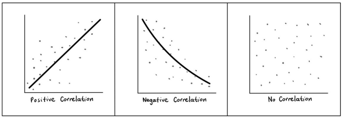
Linear and some non-linear correlations can be easily visualized.
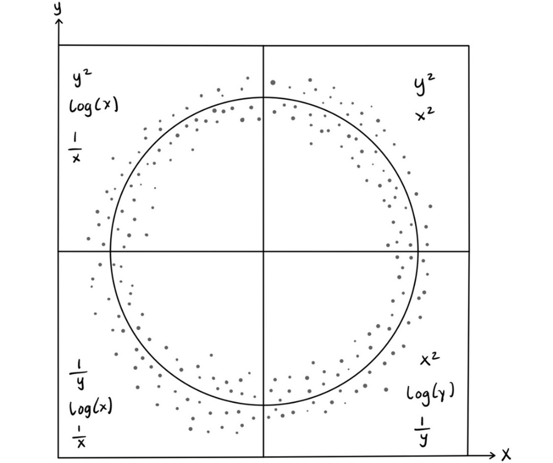
The circle of transformation recommends possible transformations to test based on the shape of the two variables you are comparing shown in a scatterplot.
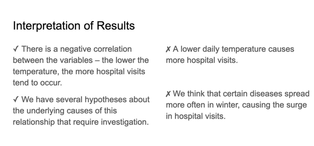
Interpretations of correlational results can provide insight into the misconceptions about their purpose and limitations.
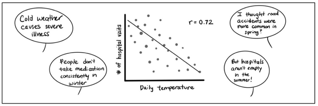
Example of a slide created to guide statistical interpretations of correlations.
Summary
- Measures of central tendency such as the mean, median, and mode are used to quickly assess the characteristics of a dataset. Each can be used in reporting to stakeholders; however, valuable information about outliers, skew, and shape can be lost if only one measure is reported.
- Measures of variability tell you how much your dataset deviates from the mean or median. These measures give you an estimate of the spread of your dataset and a first point of comparison between two or more distributions.
- Parametric statistical tests are widespread across nearly every domain of analytics. These tests make explicit assumptions about the parameters and characteristics of the underlying population distribution.
- Many parametric tests assume that your population is normally distributed. These tests require that your data can be represented as a normal distribution through trimming, transformation, or other appropriate steps.
- The majority of statistical tests leverage the p-value in the interpretation of the test coefficient. This value estimates the probability that you would observe the magnitude of group differences if there were no actual differences in the population. This value is often used as a threshold to determine statistical significance.
- Each statistical test has a minimum recommended sample size to detect an effect between groups or variables. Many tests (e.g., t-tests) also have a theoretical upper limit on your sample size before you risk generating false-positive results.
- Making inferences using regression modeling requires that you meet many of the same assumptions as tests comparing two or more groups (e.g., t-tests, ANOVAs). In addition, Pearson’s Correlation and linear regression require that your variables have a linear relationship or can be transformed into a linear relationship.
- Reporting the results of inferential statistical tests to non-technical stakeholders requires precise language to guide teams through the appropriate interpretation and the limitations of your findings.
FAQ
Which summary statistics should I review before running t-tests, ANOVAs, or correlations?
- Central tendency: mean, median, mode
- Variability: range, interquartile range (IQR), variance, standard deviation (SD)
- Sampling uncertainty: standard error of the mean (SE)
- Distribution shape: normality, skewness, kurtosis; use histograms/QQ plots/boxplots
- Outliers and group comparability: look for extreme values and similar spreads across groups
When should I use the mean, median, or mode?
- Mean: symmetric distributions with a meaningful center; sensitive to skew/outliers
- Median: skewed/asymmetric data or when outliers are present; more robust “typical” value
- Mode: categorical data, clear peaks/bins, or highlighting a disproportionately common value; pair with mean/median
What are the core assumptions of parametric tests (t-tests, ANOVAs, Pearson r, linear regression)?
- Normality (or transformable to normal) of the relevant distributions
- Independence of observations
- Equality of variances across groups (homoscedasticity)
- No extreme outliers
- Plus for regression: linearity, multivariate normality, no multicollinearity, homoscedastic residuals
How can I diagnose and address violations of parametric assumptions?
- Diagnose with histograms, QQ plots, scatterplots, residual plots, and boxplots
- Transform variables (e.g., log, square root, square) to reduce skew/nonlinearity
- Use Welch’s t-test/ANOVA when variances are unequal
- Systematically handle outliers (e.g., use IQR rules or robust stats), avoid case-by-case deletions
- Switch to non-parametric tests if data are categorical/ordinal, multimodal, strongly skewed, or not transformable
What’s the difference between standard deviation, standard error, and confidence intervals?
- Standard deviation (SD): spread of data around the sample mean
- Standard error (SE): uncertainty of the sample mean (SE = SD / sqrt(n))
- Confidence interval (CI): plausible range for the population mean
- Error bars: clearly label whether they show SD, SE, or CI; avoid implying normality with skewed data
Why can very large samples make tiny differences look statistically significant?
As sample size grows, the t-value increases while the critical value plateaus, so even trivial mean differences can be “significant.” Mitigate by pre-setting stricter alpha levels (e.g., .01/.001), reporting effect sizes (e.g., Cohen’s d), and defining domain-relevant minimum differences or CI thresholds.
How should I interpret p-values and choose an alpha level?
- P-value: probability of observing a test statistic as extreme as yours assuming the null is true
- It is not the probability your hypothesis is true or “chance caused the result”
- Choose alpha based on domain risk, study design complexity, control over confounds, and multiple comparisons; pre-specify with your hypothesis
Which correlation coefficient should I use?
- Pearson’s r: linear relationships between two continuous variables (after checking linearity)
- Spearman’s ρ or Kendall’s τ: ordinal data or monotonic, non-linear relationships
- Point-biserial: one binary and one continuous variable
- If non-linear, consider transforming variables (use the “circle of transformations”) before Pearson’s r
What checks are essential before fitting a linear regression?
- Linearity between predictors and outcome (transform if needed)
- Independence of observations
- Multicollinearity: assess correlations/VIFs and reduce redundant predictors
- Residual diagnostics: normality and homoscedasticity (use residual plots; consider weighted least squares or transforms if violated)
When should I prefer non-parametric tests, and what are common options?
- Use when data are ordinal/categorical, heavily skewed, multimodal, uniform, contain extreme outliers, or aren’t transformable
- Common choices: Mann–Whitney U (two groups), Wilcoxon signed-rank (paired), Kruskal–Wallis (3+ groups), Spearman’s ρ/Kendall’s τ (associations)

 Effective Data Analysis ebook for free
