17 Image generation

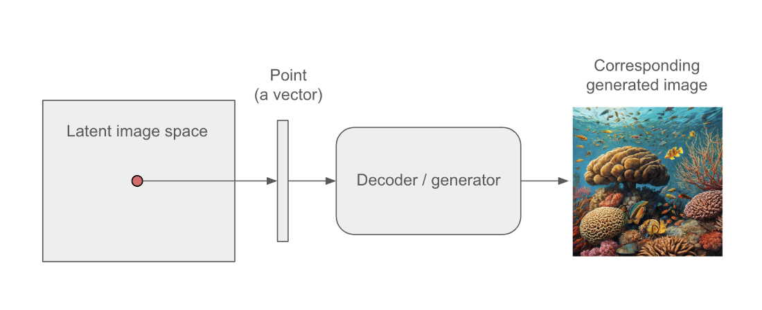
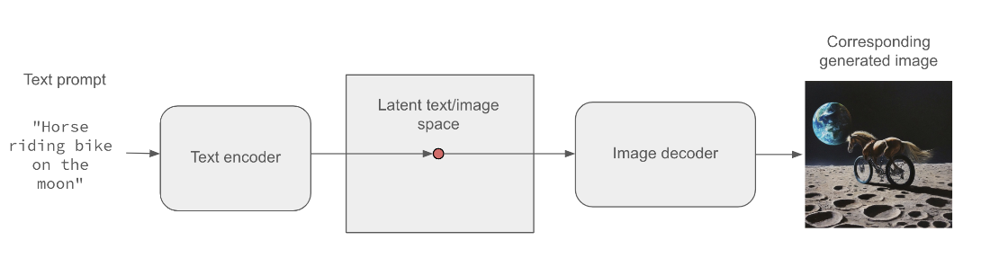
Image generation in deep learning centers on learning low-dimensional latent spaces from which new, realistic images can be sampled. A generator (or decoder) maps latent points to pixel grids, enabling interpolation between concepts and, with text-conditioning, language-guided creation. While impressive, such systems can produce artifacts due to a lack of true physical understanding. Among the main approaches, diffusion models have largely supplanted GANs for high-fidelity synthesis, while variational autoencoders (VAEs) remain valuable for interpretability and controllable latent spaces. The chapter focuses on building unconditioned VAEs and diffusion models from scratch, then demonstrates how to leverage a pretrained text-to-image model and analyze its latent space.

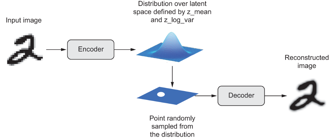
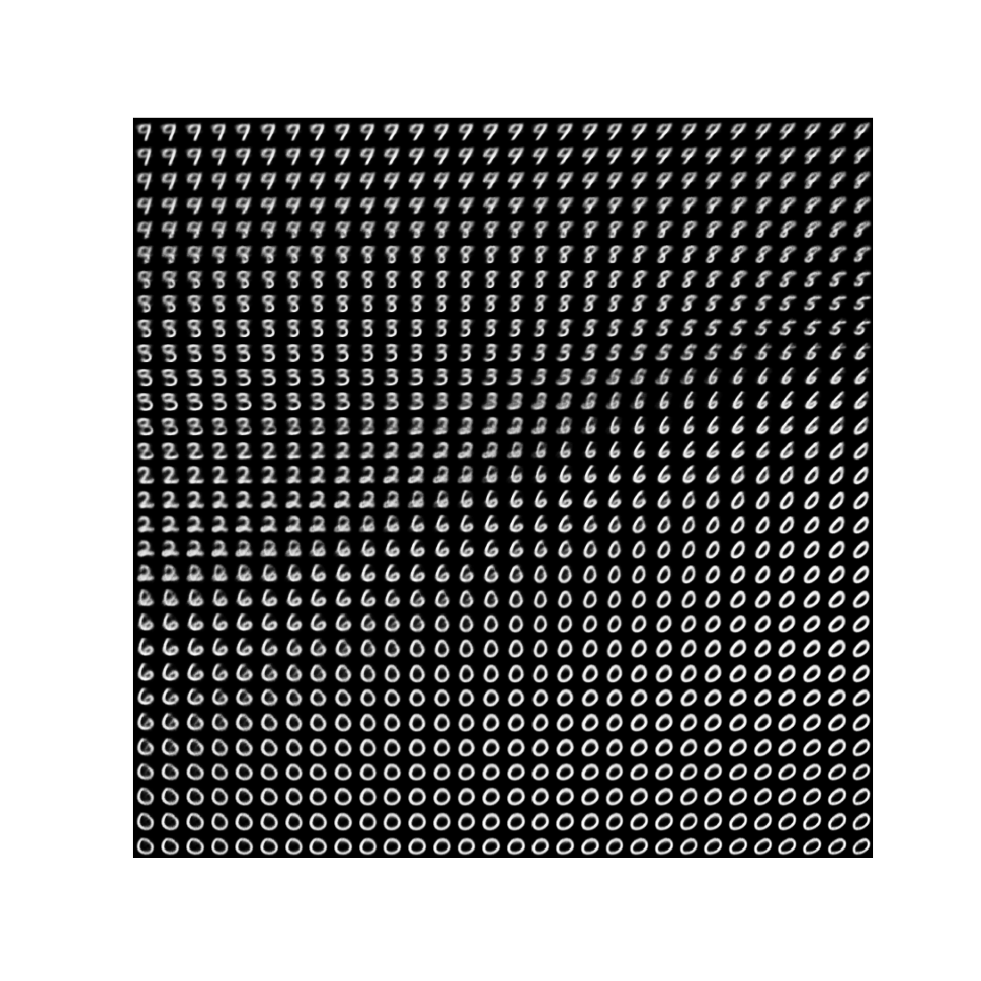
VAEs extend classical autoencoders by encoding inputs into the parameters of a probability distribution (mean and variance) and decoding a sampled latent vector back to the original domain. This stochastic “reparameterization” encourages smooth, well-structured latent manifolds where nearby points decode to similar images, making the space amenable to semantic manipulation. Training optimizes a reconstruction loss plus a KL-divergence regularizer that nudges the latent distribution toward a standard normal. A compact Keras implementation illustrates the full workflow on MNIST digits, culminating in latent-space sampling that smoothly morphs one digit into another and reveals meaningful directions (concept vectors) across the manifold.

Diffusion models recast generation as iterative denoising: starting from pure noise, a shared denoiser (often a U-Net) removes noise step by step according to a diffusion time and schedule (e.g., cosine) that control signal and noise rates. Training teaches the denoiser to predict noise masks under varying noise levels (with normalized inputs and simple losses), while inference repeatedly denoises to produce crisp images. The chapter then extends the idea to text-to-image by conditioning denoising on text embeddings, and shows practical use of a pretrained Stable Diffusion model, including negative prompts and step control. Finally, it explores the text latent space via spherical interpolation between prompts, visually demonstrating how deep models act as powerful interpolation machines across language and vision.

Using a latent vector space to sample new images

Language-guided image generation

An autoencoder: mapping an input x to a compressed representation and then decoding it back as x’

A VAE maps an image to two vectors, z_mean and z_log_sigma, which define a probability distribution over the latent space, used to sample a latent point to decode.

Grid of digits decoded from the latent space

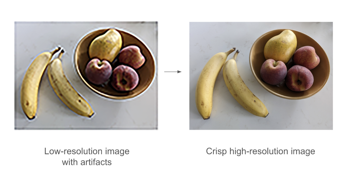
Image super-resolution

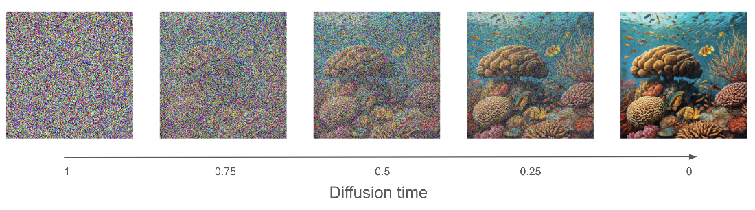
Reverse diffusion: turning pure noise into an image via repeated denoising

An example image from the Oxford Flowers dataset.

Our U-Net style denoising autoencoder architecture

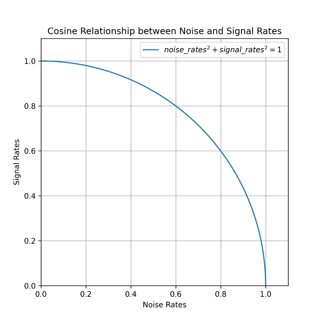
Cosine relationship between noise rates and signal rates

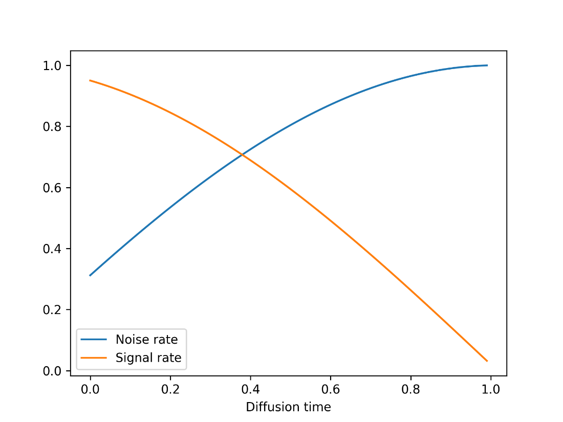
Our cosine diffusion schedule

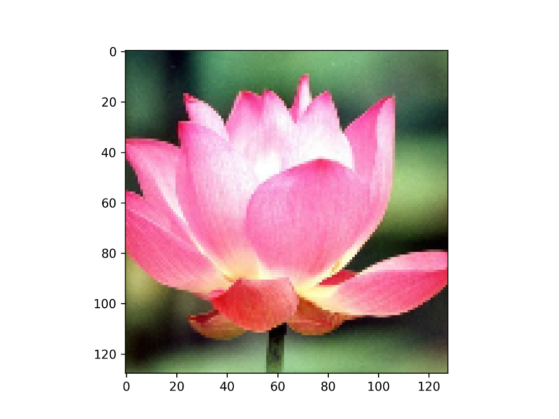
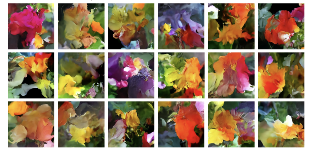
Examples of generated flowers

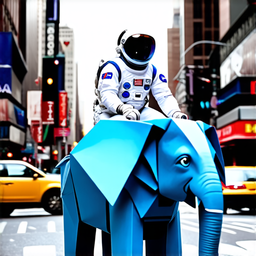
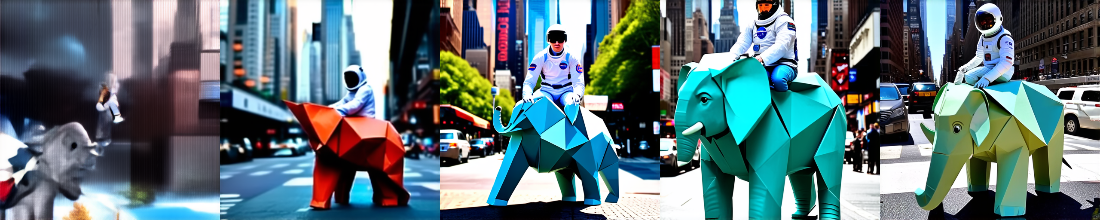
An example output from our Stable Diffusion model.

Controlling the number of diffusion steps.

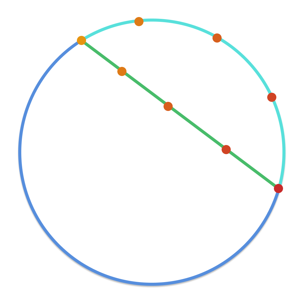
Spherical interpolation keeps us close to the surface of our manifold.

Interpolating between two prompts and generating outputs.

• Image generation with deep learning is done by learning latent spaces that capture statistical information about a dataset of images. By sampling and decoding points from the latent space, you can generate never-before-seen images. There are three major tools to do this: VAEs, diffusion models, and GANs.
• VAEs result in highly structured, continuous latent representations. For this reason, they work well for doing all sorts of image editing in latent space: face swapping, turning a frowning face into a smiling face, and so on. They also work nicely for doing latent-space-based animations, such as animating a walk along a cross section of the latent space, showing a starting image slowly morphing into different images in a continuous way.
• Diffusion models result in very realistic outputs and are the dominant method of image generation today. They work by repeatedly denoising an image, starting from pure noise. They can easily be conditioned on text captions in order to create text-to-image models.
• Stable Diffusion 3 is a state-of-the-art pretrained text-to-image model that you can use to create highly realistic images of your own.
• The visual latent space learned by such text-to-image diffusion models is fundamentally interpolative. You can see this by interpolating between the text embeddings used as inputs to the diffusion process, and achieve a smooth interpolation between images as output.

FAQ