4 Solubility Deep Dive with Linear Models

Drug solubility is presented as a central problem in pharmaceutical modeling because it strongly influences bioavailability, especially for oral drugs that must dissolve and survive the gastrointestinal environment before reaching circulation. The chapter uses solubility as a practical case study for linear models, showing how experimentally measured values can be paired with molecular descriptors to build predictive models that help prioritize compounds with better chances of success. It also emphasizes that real solubility data can be noisy, inconsistent across studies, and populated by outliers, so careful dataset inspection is essential before modeling.

The workflow begins with scaffold-based splitting of the AqSolDB dataset to avoid overly optimistic evaluation caused by structurally similar molecules appearing in both train and test sets. The text then walks through descriptor calculation, correlation analysis, and feature engineering, using properties such as molecular weight, logP, hydrogen-bond donors, and aromatic proportion. It shows how some descriptors correlate strongly with solubility while others add little signal, and it introduces applicability domain reasoning so the model is only trusted within chemical space similar to the training data. A baseline linear regression is then fitted, and the chapter explains the underlying learning mechanics, including ordinary least squares, gradient descent, feature scaling, and the use of MSE, MAE, and R² for evaluation.

After establishing the basics, the chapter surveys several Scikit-Learn linear approaches, including Ridge regression, sequential feature selection, and more robust SGD-based models such as RANSAC and support vector regression. It compares these against an ESOL benchmark and a y-scrambled baseline to test whether the models are truly learning meaningful structure rather than chance patterns. The strongest model uses an epsilon-insensitive loss with polynomial features, inverse learning-rate scaling, and early stopping, giving the best test performance among the methods examined. The chapter closes by connecting these results to the bias-variance trade-off, showing how learning curves and validation curves reveal when a model is underfitting, overfitting, or balanced well enough to generalize.

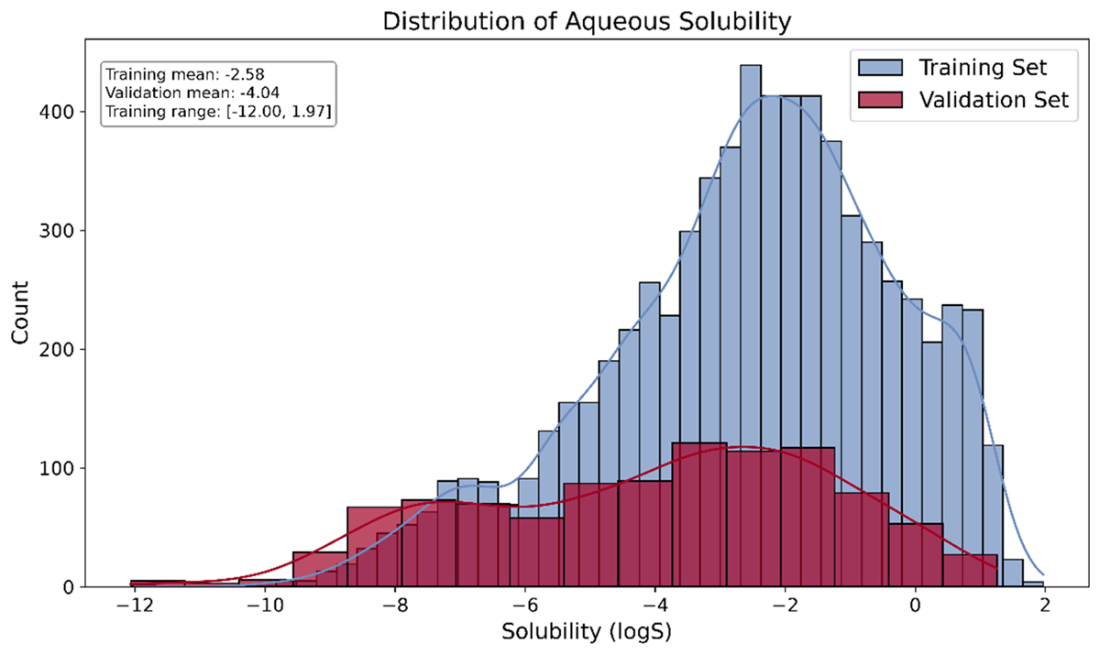
Comparison of solubility distributions for train and validation data sets.

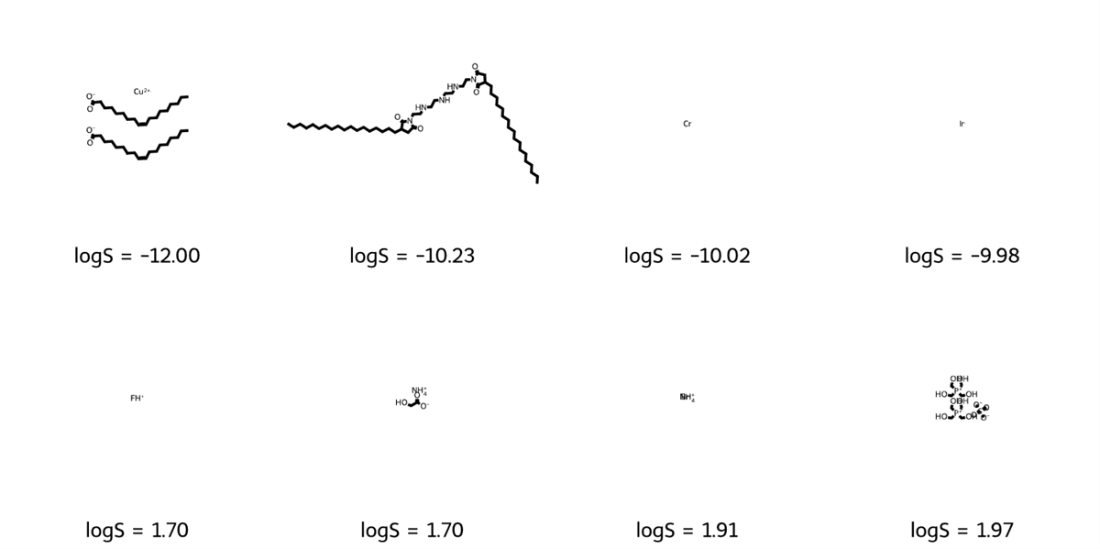
The least soluble molecules (top row) and the most soluble molecules (bottom row) in the training data set.

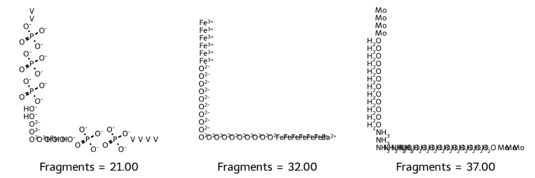
Three molecules with the greatest number of fragments in the training data set.

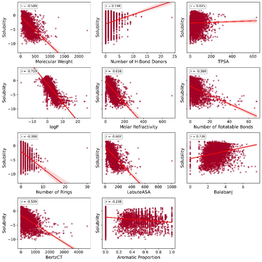
Scatterplots of each descriptor with respect to solubility, our target variable.

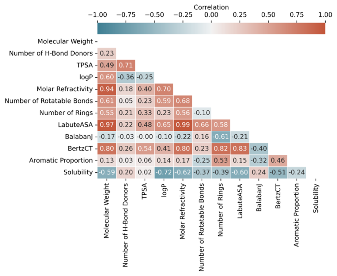
Correlation heatmap for each pair of descriptors and solubility.

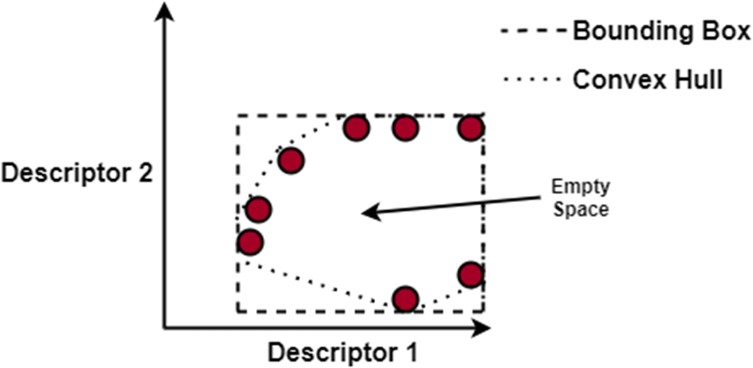
Estimated model AD based off of regions defined by the bounding box (dashed line) and convex hull (dotted line) methods.

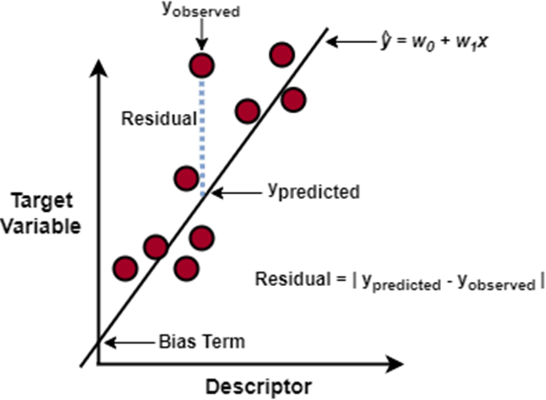
Example depiction of simple linear regression

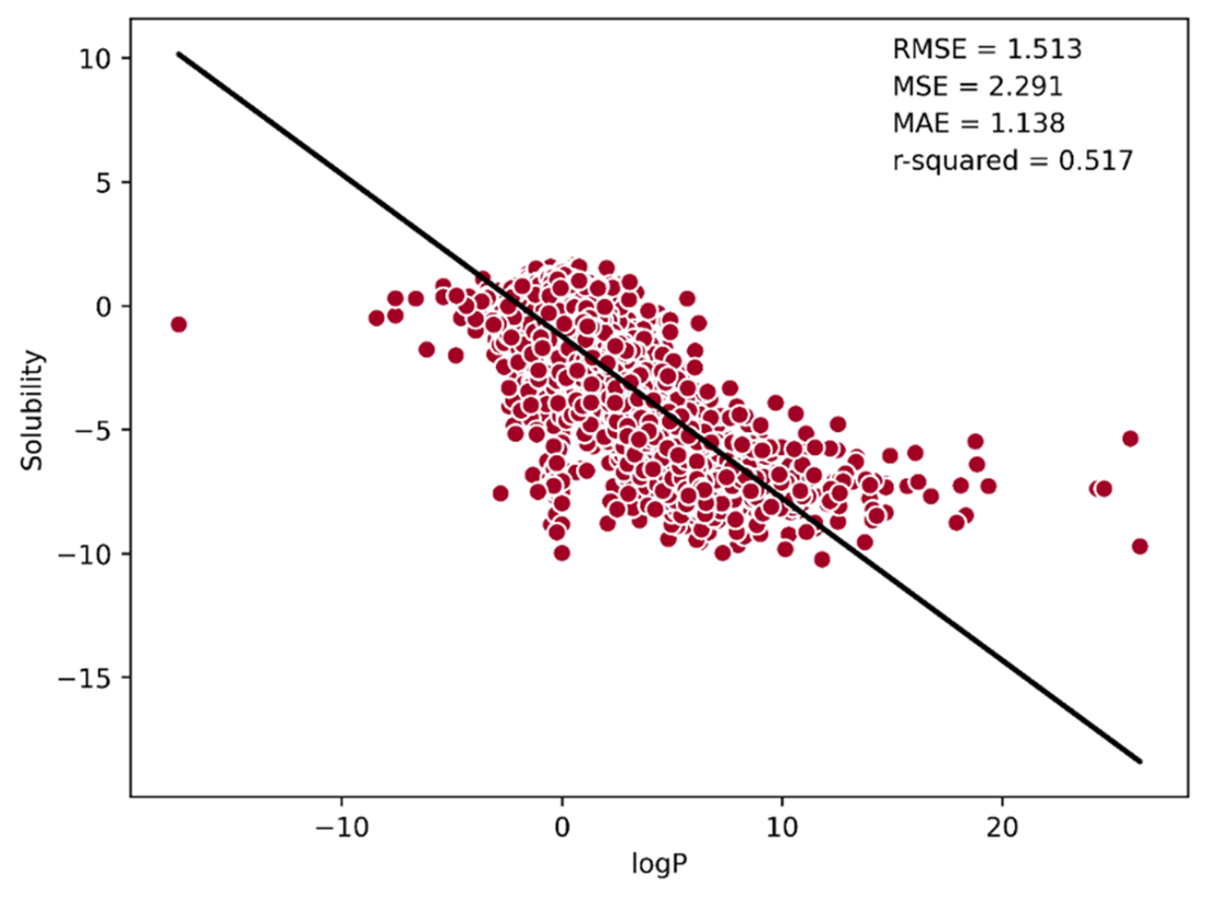
Performance of our simple linear regression model on the training data.

Adjusting the model’s weights results in different regression lines, ideally minimizing the MSE.

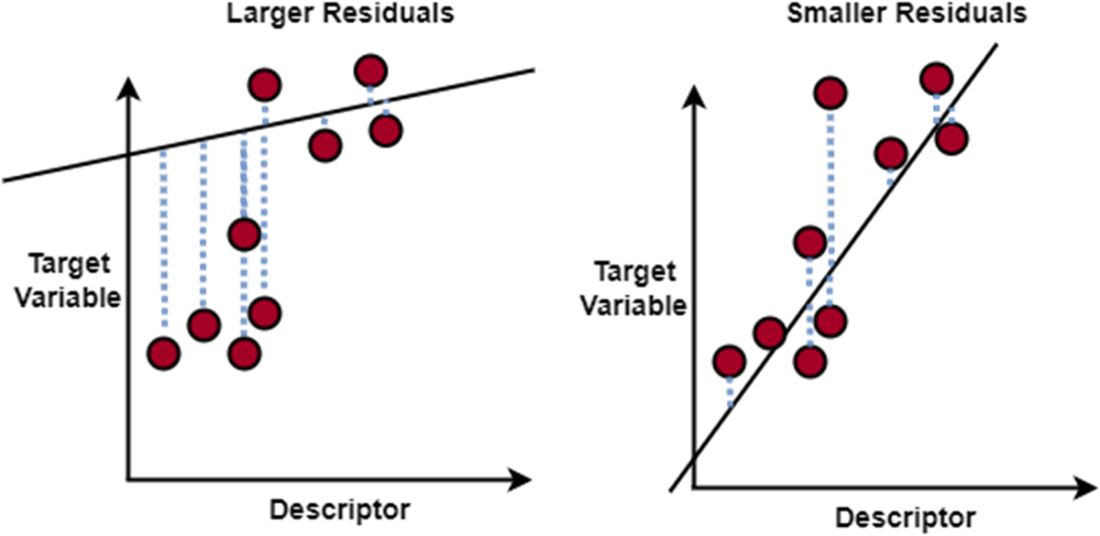
Example cost function surface we may navigate with gradient descent.

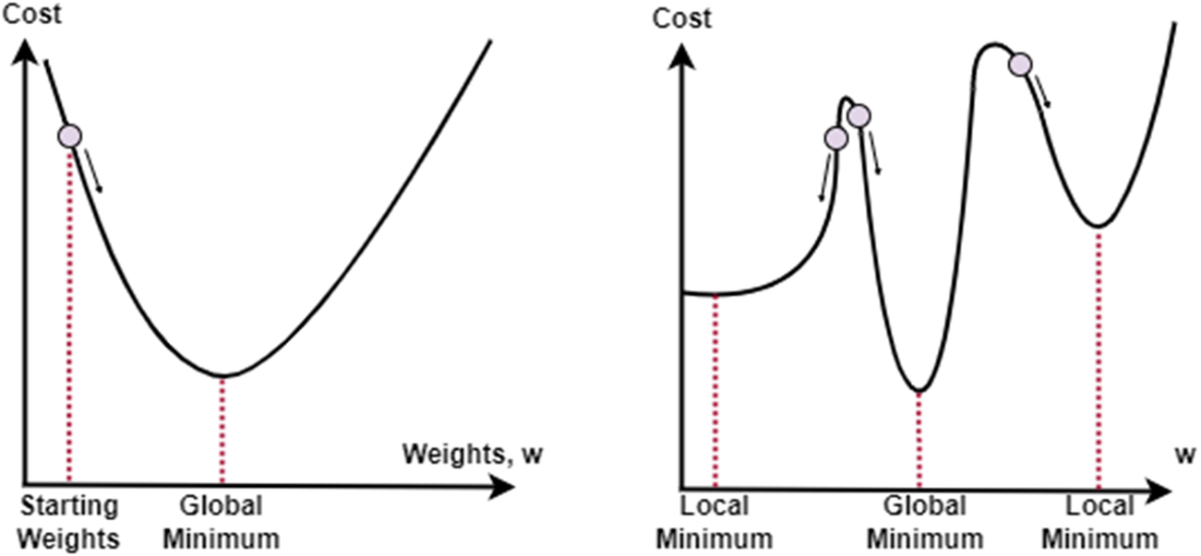
Impact of learning step size on the ability for gradient descent to converge.

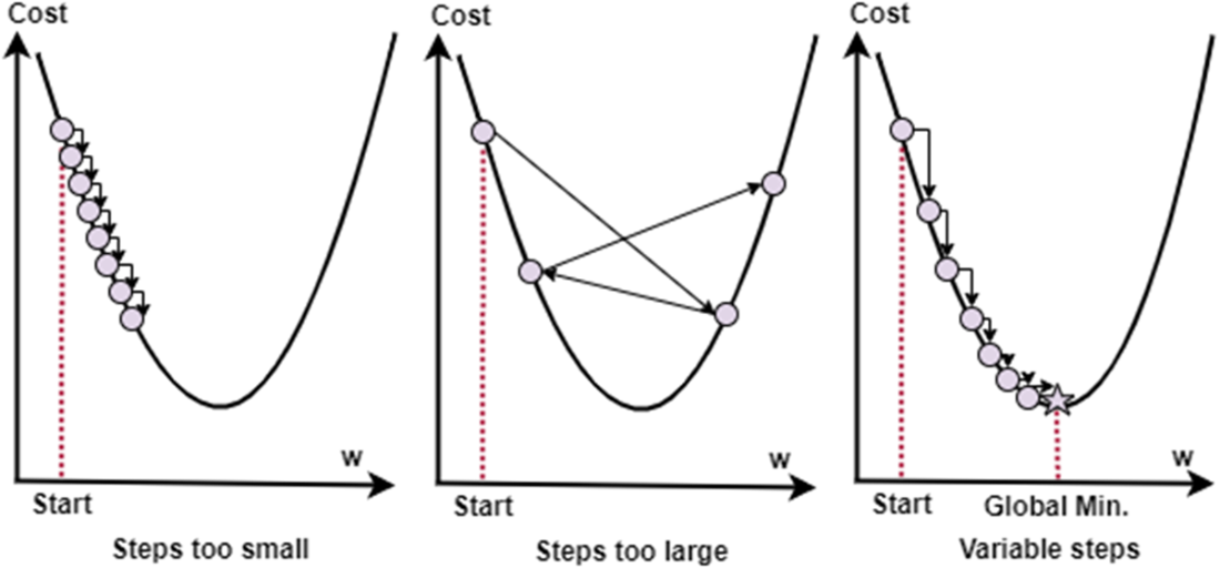
A combination of gradient descent stopping criterion works best to mitigate early termination when hitting the first plateau.

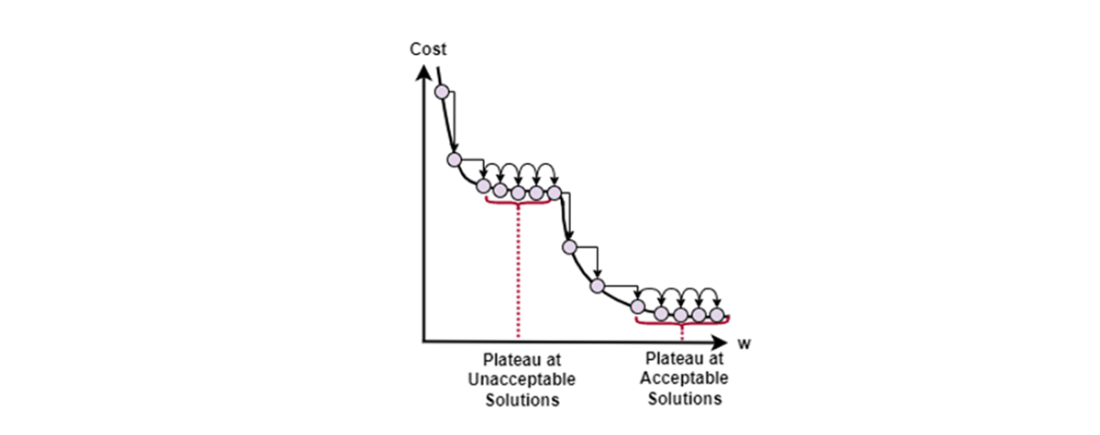
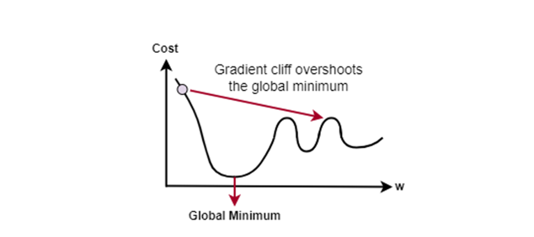
Gradient cliffs impact converging to an optimal minimum of model weights.

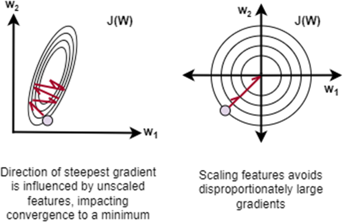
Effect of feature scaling on the convergence of gradient descent.

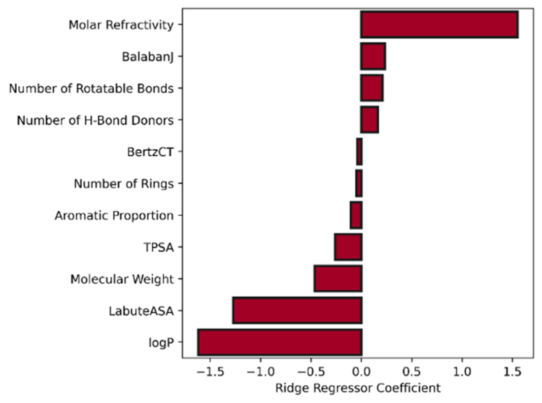
Ridge regressor coefficients for each descriptor.

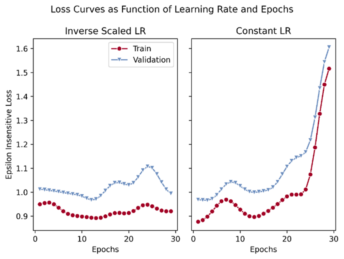
Loss curves as a function of learning rate schedular and number of epochs.

Impact of model complexity on the fitted model’s training and testing performance.

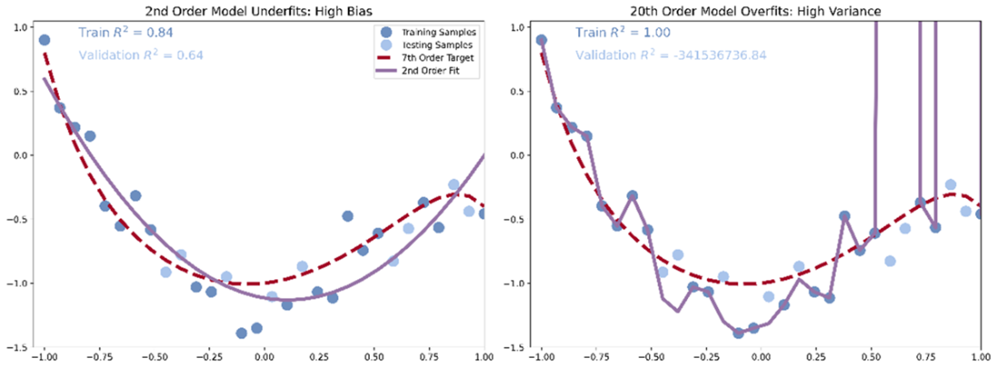
How high bias or high variance impact a model’s sensitivity to the training data it learns from.

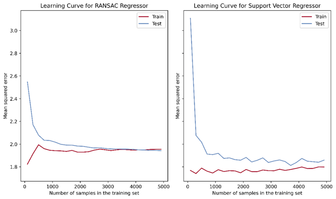
Learning curves for RANSAC and SVR models.

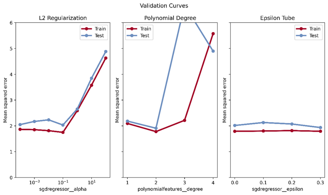
Validation curves for SVR and preprocessing hyperparameters.

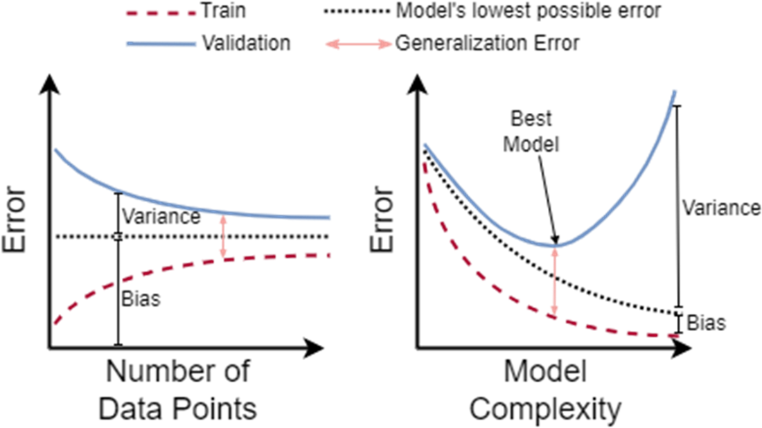
How different errors (train, validation, generalization) and bias and variance change as a function of the number of data points (left, learning curve) or the model complexity (right, validation curve).

• Using AqSolDB, we explored another fundamental problem to drug discovery – characterizing a molecule’s solubility. Poor solubility can lead to reduced absorption, necessitating higher drug doses and potentially causing adverse effects, while good solubility can enhance a drug's therapeutic profile.
• We reviewed the underlying mechanics of linear models through the specifics of linear regression. We explored closed-form (normal equation) and iterative (gradient descent) solutions in determining the optimal set of linear weights.
• Gradient descent has additional variants in the form of batch, mini-batch, and stochastic gradient descent. These variants have implications on runtime and memory, as well as convergence on a performative set of weights. Additional peculiarities to consider when using gradient descent are the learning rate, convergence criteria, gradient clipping, and feature scaling.
• We gained exposure to a greater breadth of linear models that are easily accessible in Scikit-Learn. Expanding our toolkit beyond linear regression, RANSAC is an iterative method used for robust estimation and model fitting in the presence of outliers and SVR finds a hyperplane that fits the data while allowing for a margin of error (epsilon-tube) around the predicted values.
• A model with high bias makes overly simplistic assumptions about the target function’s complexity and is incapable of capturing the underlying patterns in the training data. A more complex model with more learnable parameters may have smaller bias that allows it to better approximate the target function, but the additional complexity makes it harder to find and pin down the best approximation.

FAQ