11 Graph Neural Networks for Predicting Drug-Target Affinity

This chapter introduces drug-target affinity prediction as a core problem in virtual screening, where the goal is to estimate how strongly a candidate molecule binds to a protein target so researchers can prioritize the most promising pairs for experimentation. It explains why sequence-only representations can miss important structural and topological information, and motivates a graph-based approach that better matches the chemistry of molecules and the spatial organization of proteins. The discussion is anchored in benchmark datasets such as DAVIS and KIBA, while also highlighting practical issues like noise, imbalance, sparsity, and the difference between warm-start and cold-start evaluation settings.

The main technical contribution is a dual-graph modeling pipeline that converts both drugs and proteins into graph representations with informative node features. Small molecules are built from SMILES strings into atom-bond graphs, with atom-level descriptors such as symbol, degree, hydrogen count, valence, and aromaticity. Proteins are represented as residue interaction graphs using contact maps derived from structural or predicted information, and each residue is encoded with biochemical properties plus evolutionary signals from PSSMs computed from multiple sequence alignments. These design choices aim to preserve meaningful structural context while keeping the data usable for neural networks.

Once the graphs are prepared, the chapter explains the foundations of graph neural networks and shows how message passing, pooling, and readout operations turn variable-size graphs into fixed-size embeddings. It then builds a symmetric dual-stream architecture in which the drug and protein graphs are processed separately by GNN encoders, pooled into embeddings, concatenated, and passed through a prediction head to estimate binding affinity. The chapter also compares GCN, GAT, and GIN variants, trains and evaluates them on benchmark data, and interprets results using MSE, Pearson correlation, CI, and rm², concluding that graph-based models are useful for ranking and prioritizing candidates in real drug discovery workflows.

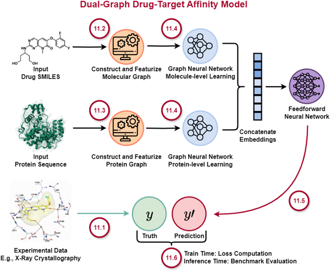
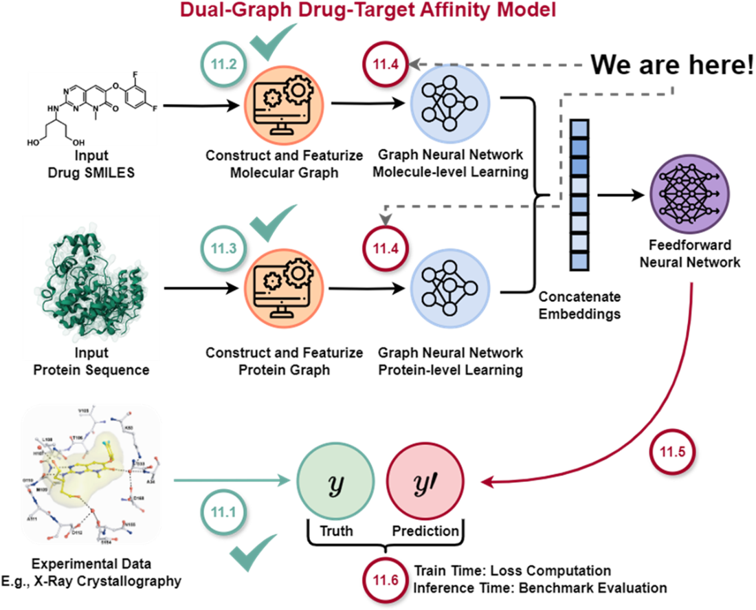
Architecture of a Dual-Graph Model for Drug-Target Affinity Prediction. In section 11.1, we’ll familiarize ourselves with the problem of drug-target affinity prediction so we can better understand our objective for this chapter, why we need to work with both molecule and protein data inputs, why graph neural networks offer an advantageous approach over alternatives, and what benchmarks we’ll be using to guide model development. Section 11.2 and 11.3 detail how we can transform textual representations of molecules and proteins into rich, graph-based representations. In section 11.4, we’ll introduce the core learning engine, graph neural networks, that facilitate learning on graphs. Section 11.5 combines the previous sections to show the full DGraphDTA dual-stream architecture implementation, which we’ll train and later evaluate in section 11.6. The illustrated inputs (SMILES, protein sequence, experimental data) are based on a real result from [3] concerning development of a series of p38α inhibitors for rheumatoid arthritis.

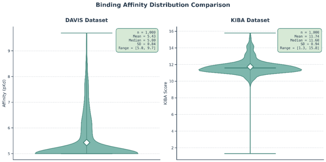
Distribution of pKd Affinity Values in the DAVIS Dataset and KIBA scores in the KIBA Dataset. For the DAVIS dataset, we observe a very large, sharp peak visible at the y-value of 5, with a much smaller, broader distribution of values between 6 and 10.

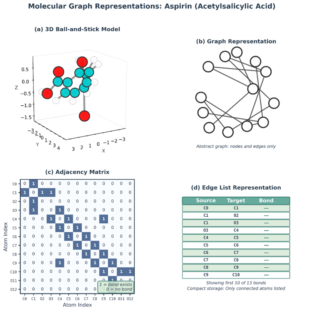
Graphs contain multitudes. Aspirin represented as a graph across multiple formats: 1) 3D ball-and-stick model, 2) Graph representation with nodes and edges, 3) Adjacency matrix representation, 4) Edge list representation.

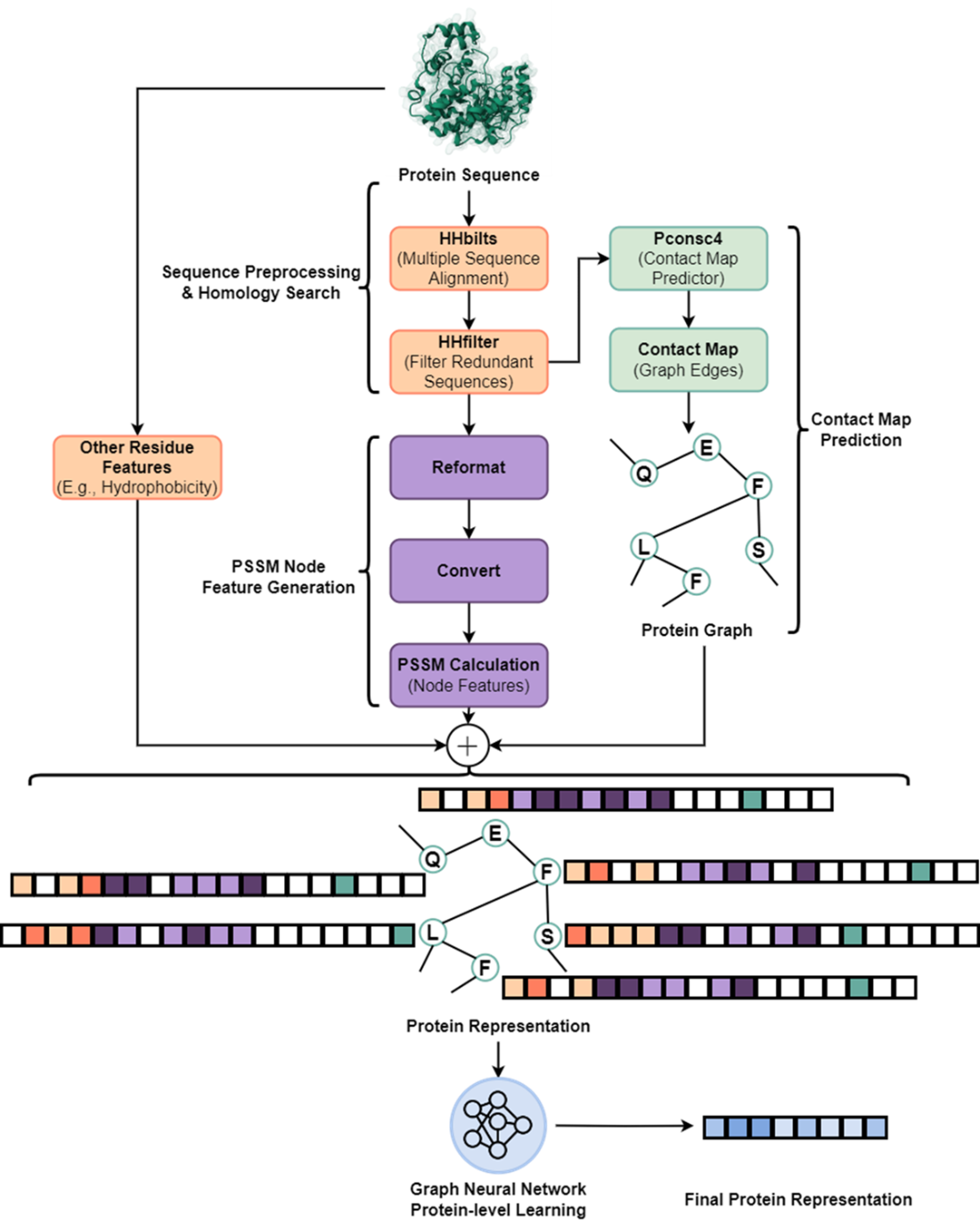
The Protein Preprocessing and Feature Generation Pipeline. The process begins with a single protein sequence. A multiple sequence alignment (MSA) is generated with HHblits and subsequently filtered by HHfilter. The pipeline then splits into two parallel branches: (1) the filtered MSA is fed into Pconsc4 to predict a contact map, which will define the protein graph's edges, and (2) the MSA is used to calculate a Position-Specific Scoring Matrix (PSSM), which serves as a primary feature for the graph's nodes. All three of these feature computation branches can occur in parallel after sequence preprocessing via HHbilts and HHfilter. Once ready, the contact map, PSSM, and other protein features are combined to construct the full protein graph, which is then processed in aggregate by a GNN to generate the final protein representation. The feature vectors are represented at 3 features to 1 cell ratio.

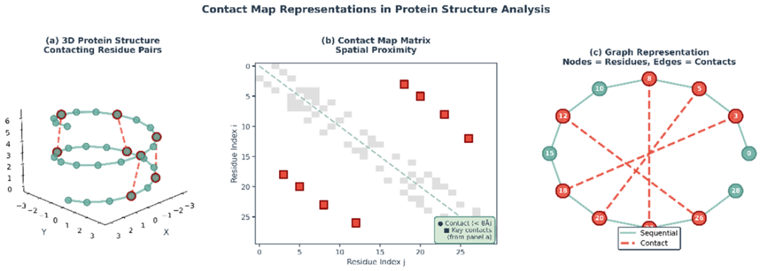
Transforming a Protein's 3D Structure into a 2D Graph. Converting a protein's spatial information into a graph representation. (a) A simplified 3D protein structure with dashed lines connecting amino acid residues that are in close spatial proximity (a 'contact'). (b) Spatial information is translated into a contact map, which is a 2D matrix. A point at (i, j) is marked if residue i and residue j are in contact, serving as an adjacency matrix for the graph. (c) The contact map is used to construct a graph where the amino acid residues are the nodes and the contacts are the edges. This graph captures the key residue interactions in a format that is invariant to the protein's rotation and translation in 3D space.

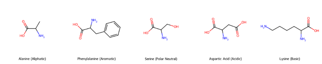
Chemical Diversity of Amino Acid Side Chains. The figure displays five amino acids, each representing one of the major chemical classes. From left to right: Alanine, an aliphatic amino acid with a simple methyl side chain; Phenylalanine, an aromatic amino acid containing a phenyl group; Serine, a polar neutral amino acid with a hydroxyl group; Aspartic Acid, an acidic amino acid with a carboxyl group; and Lysine, a basic amino acid with an amino group. These diverse side chains are fundamental to determining protein structure and its interactions with other molecules.

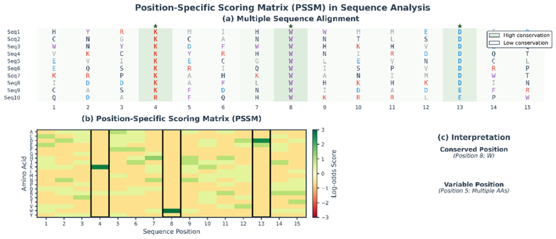
Derivation and Interpretation of a PSSM. (a) MSA of related protein sequences. Each column represents a position in the sequence. Some positions are highly conserved across sequences (e.g., position 8, dominated by Tryptophan, W), indicating functional or structural importance. Other positions are more variable (e.g., position 5). (b) The PSSM derived from the MSA. It is a matrix of log-odds scores where each cell quantifies the likelihood of a specific amino acid occurring at a specific position compared to its background frequency. The highly conserved Tryptophan at position 8 has a large positive score (dark green). (c) This quantitative representation allows for easy interpretation, clearly distinguishing conserved positions from variable ones.

We are now ready to proceed to the theoretical mechanisms that underlie graph neural networks!

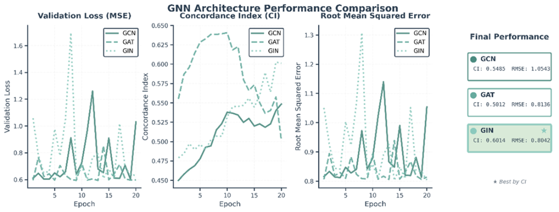
Performance comparison of three GNN architectures trained for 20 epochs on a subset of the DAVIS dataset. The plots track three key validation metrics over the course of training: (left) Validation Loss (Mean Squared Error), (center) Concordance Index (CI), and (right) Root Mean Squared Error (RMSE). The final performance panel on the far right shows that the GIN architecture achieved the best performance, with the highest Concordance Index (CI = 0.6014). However, notice GAT’s early performance superiority before overfitting – in practice we would use an earlier checkpoint than the 20 epoch version.

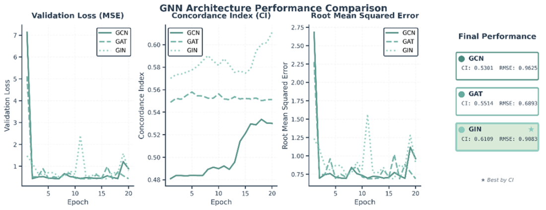
Performance comparison of three GNN architectures trained for 20 epochs on a subset of the KIBA dataset. The plots track three key validation metrics over the course of training: (left) Validation Loss (Mean Squared Error), (center) Concordance Index (CI), and (right) Root Mean Squared Error (RMSE). The final performance panel on the far right shows that the GIN architecture achieved the best performance, with the highest Concordance Index (CI = 0.6109).

• Graph representations provide a natural and powerful way to encode molecular structure. Unlike fixed-length feature vectors that must be hand-crafted for each application, graphs directly capture the connectivity patterns in molecules and proteins. Graph representations align with the natural structure of molecules and proteins. Molecules are graphs where atoms are nodes and bonds are edges. Proteins, while sequentially synthesized, fold into three-dimensional structures where spatial proximity matters more than sequential proximity. Representing both as graphs allows neural networks to learn from local structural patterns rather than having to infer structure from sequential notation.
• The message passing algorithm is the core engine that allows GNNs to learn context-aware representations of nodes by iteratively aggregating information from their local neighborhoods. Different GNN layers (GCN, GAT, GIN) offer a trade-off between computational complexity and expressive power, with GIN often providing the best performance on tasks requiring high structural sensitivity.
• The PyTorch Geometric library provides the essential, high-performance tools for building complex, graph-based deep learning models for drug discovery, including handling the batching of variable-sized graphs.
• The dual-stream architecture embodies an important principle in machine learning: when dealing with heterogeneous data types, allowing specialized processing of each type before fusion often outperforms mixed processing from the start. Drugs and proteins have fundamentally different structures and scales, and the dual-stream design respects these differences.
• Careful feature engineering remains important even in deep learning. While the GNN learns complex derived features, providing informative initial features (atomic properties, residue biochemistry) gives the model a strong starting point and improves sample efficiency. For molecules, encoding atom type, degree, valence, and aromaticity gives the network a head start. For proteins, combining one-hot encoding, evolutionary information from PSSMs, and biochemical properties creates a comprehensive representation.
• Looking forward, the intersection of graph neural networks and computational biology remains an active and exciting research area. Improvements in protein structure prediction, particularly through AlphaFold2 and related methods, provide increasingly accurate structural information that GNNs can exploit. Growing datasets of drug-target interactions, molecular properties, and chemical reactions provide more training data for learning better representations. Novel architectures that incorporate physical constraints, symmetries, and domain knowledge promise to combine the flexibility of machine learning with the rigor of biophysics.
• Evolutionary information provides powerful signal for protein structure prediction. Multiple sequence alignments contain correlated mutations that reveal spatial contacts. Methods like Pconsc4 leverage this signal through deep learning to predict contact maps with high accuracy. These predicted contact maps, though not perfect, provide sufficient structural information to substantially improve binding affinity prediction.
• The broader lesson extends beyond drug discovery. Many problems involve structured data (social networks, knowledge graphs, molecular interaction networks) where GNNs can provide effective representations. The principles illustrated in constructing meaningful graph structures, engineering informative node features, designing architectures appropriate to the graph type, and combining heterogeneous inputs through dual-branch networks apply broadly across domains.

FAQ