Appendix I. Diffusion & Flow Matching with FlowMol3, DiffSBDD, RFdiffusion, & Boltz-2
De novo molecular design has moved beyond one-shot latent decoders because generating valid three-dimensional chemistry is too delicate to trust to a single pass. Instead of compressing molecules into a latent map and decoding them all at once, the chapter presents a newer paradigm: start from noise and refine gradually, letting a model make many small corrections until a coherent structure emerges. This iterative view is introduced as the natural next step for drug design, where validity, novelty, synthesis feasibility, and safety can all matter at once.
The chapter first explains diffusion as learning to reverse a noising process: clean data is systematically corrupted, then a neural network is trained to predict the noise so the sample can be denoised step by step. In the two-moons toy example, this works well but becomes expensive because good samples require many reverse steps. Flow matching is then presented as a generalization that learns a velocity field instead of a stochastic reverse process, allowing samples to travel along much straighter paths and reach similar or better quality in far fewer steps. The toy experiments make the tradeoff clear: diffusion is flexible but step-hungry, while flow matching preserves quality with much better sampling efficiency.
That efficiency is then carried into real drug-discovery tasks. FlowMol3 shows how multi-modal flow matching can generate valid 3D molecules by combining continuous coordinate flow with discrete atom and bond updates, producing drug-like compounds with good QED and synthetic accessibility in only tens of steps. DiffSBDD extends diffusion into structure-based design by conditioning on a protein pocket, enabling ligand generation, optimization, and scaffold inpainting inside a target site, though sometimes at the cost of internal strain. RFdiffusion demonstrates the mirror-image task of designing a protein around a ligand, and Boltz-2 is used as a downstream triage layer to score generated complexes by predicted binding and affinity. Together, these models form a composable pipeline in which generation, conditioning, and screening can be chained into a practical workflow for interactive AI-driven drug discovery.
Figure I.1 On the left, a single latent point is fed through a decoder and emerges as a finished molecule — fast, but with no way to correct a flawed output. In the center, the new paradigm this chapter develops: generation as iterative refinement, where a sample starts as pure noise and is pushed step by step, through a long chain of small denoising moves, until it becomes structured data. The panel contrasts diffusion's many-step stochastic reversal with flow matching's straighter, fewer-step path. On the right, the destinations we reach with pretrained models: a validated 3-D drug-like molecule generated unconditionally (I.4) and a ligand designed to fit a protein binding pocket (I.5).
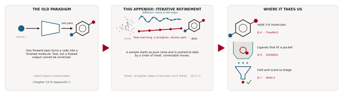
Figure I.2 The forward process applied to 2,000 points drawn from the two-moons target, shown at six increasing noise levels (t = 0, 25, 50, 100, 150, 200) of a 200-step cosine schedule. At t = 0 the two interleaving crescents are perfectly sharp. As t grows the points scatter outward and the crescents thicken and merge, the structure visibly dissolving; by the final panel the distribution is an isotropic Gaussian blob from which the original shape cannot be recovered by eye. Each panel is produced by the single q_sample call from Listing I.1.

Figure I.3 The reverse process on the two-moons target, in two parts. Panel (a) shows the full 200-step reverse process succeeding: 1,500 points are carried from a Gaussian starting cloud (purple) through intermediate denoising snapshots to their final resting places on the two crescents (yellow), the color tracking progress through the run. Panel (b) is the catch — the same trained model sampled under shrinking step budgets of 200, 32, 16, 8, and 4 reverse steps, with the energy distance to the target printed beneath each. At 200 and 32 steps the moons are crisp (energy ≈ 0.005, shown in blue); by 8 steps they fray and by 4 steps the structure collapses into a diffuse blob (shown in red). The panel is the visual proof that diffusion's sample quality is tied to its step count, and it sets up the central question the rest of the chapter answers: can we keep the quality while paying for far fewer steps?
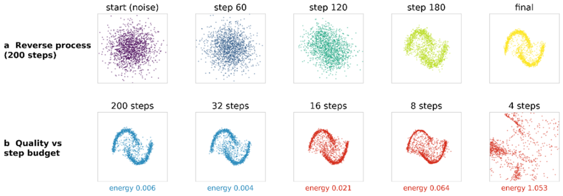
Figure I.4 The left panel plots energy distance (lower is better; the dashed band marks the roughly 0.01 high-quality region) against the number of sampling steps for three samplers on the same two-moons target. Flow matching (crimson) reaches the high-quality band at 8 steps and the diffusion model's ancestral sampler (slate) needs 32, the roughly fourfold difference this section leads with. The third curve is DDIM at eta equal to zero (grey), the deterministic probability-flow ODE for the very same trained diffusion network on the very same noise ladder, and it never reaches the band at all, still at 0.073 after exhausting all two hundred noise levels the schedule provides. The right-hand panels show the generated points at a matched budget of 8 steps. Because DDIM and ancestral sampling share a network and differ only in whether noise is injected, the third curve isolates path geometry from sampling stochasticity: the step advantage is not an artifact of comparing a stochastic sampler against a deterministic one.
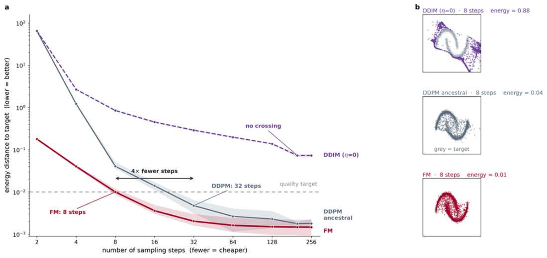
Figure I.5 Property profile of the FlowMol3-generated molecules. Each panel shows one physicochemical property across the generated batch: the quantitative estimate of drug-likeness (QED), the synthetic accessibility (SA) score, molecular weight, and calculated lipophilicity (cLogP), with shaded bands marking the ranges typical of orally administered drugs. The molecules cluster inside those bands: a mean QED of 0.72 puts the batch in drug-like territory, and a mean SA score of 2.43 says they should be straightforward to synthesize. Molecular weight and cLogP likewise fall within the conventional oral-drug windows, so the model is producing chemically reasonable, drug-like molecules rather than merely valid graphs.
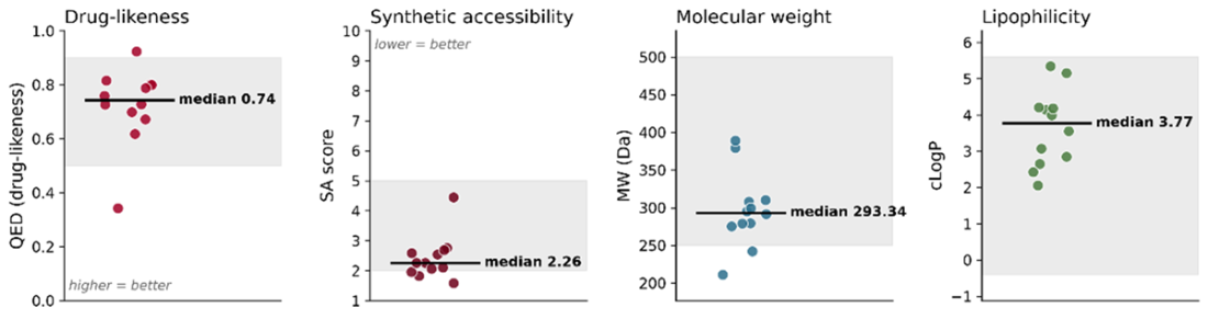
Figure I.6 The step-count thesis on molecules. The plot tracks the chemical validity of FlowMol3-generated molecules, alongside their synthetic accessibility, as the number of integration steps increases from 10 to 250, holding the random prior fixed so that only the step budget changes. Validity rises sharply (41.7% at 10 steps, 83.3% at 25 steps) and saturates at 100% by 50 steps, after which the curve is flat through 100 and 250 steps. Roughly 50 steps is enough to generate fully valid drug-like molecules.
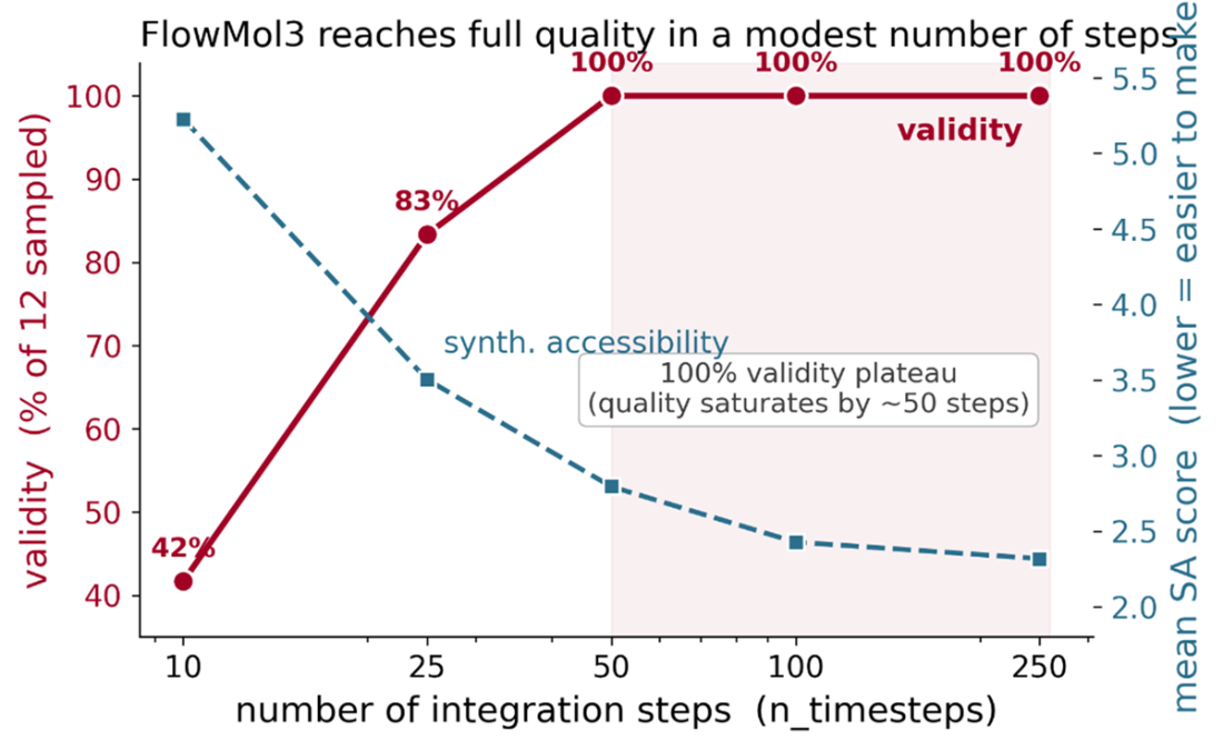
Figure I.7 Physical plausibility of the generated molecules, a stricter bar than the graph validity reported above. Panel (a) gives the fraction of each batch passing PoseBusters' intramolecular checks: FlowMol3's twelve molecules (slate) pass all of them, while DiffSBDD's twenty (crimson) fail bond angles on three molecules and bond length s on two. Panel (b) shows that every ligand-to-protein check passes for the DiffSBDD batch, so the molecules are placed cleanly against the receptor even where their internal geometry is strained. Panel (c) plots UFF strain energy on a log scale, the difference between each pose's energy and that of a relaxed conformer ensemble: the DiffSBDD median of 134 kcal/mol sits roughly 350 times the co-crystal caffeine reference of 0.39, with five molecules above 300, while FlowMol3's median of 8 is far closer to the reference. The pattern to take away is that a pocket-conditioned generator can satisfy the protein and still hand you a strained molecule.
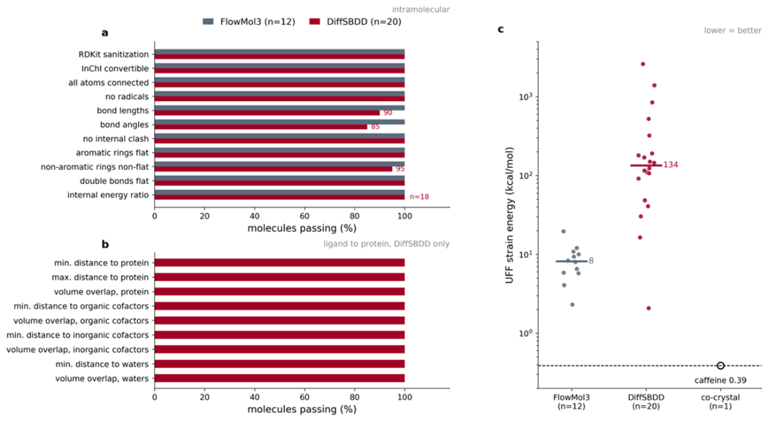
Figure I.8 Profile of the twenty pocket-conditioned ligands DiffSBDD generated for the adenosine A2A receptor, with each molecule plotted as a single point and caffeine, the reference ligand, marked as a dashed line for comparison. Panel (a) shows drug-likeness (QED, where higher is better): the generated set has a median QED of 0.60, edging above caffeine's 0.54, with the best candidates climbing toward 0.8. Panel (b) shows synthetic accessibility (SA score, where lower is easier to make): the median sits at 4.25, meaningfully harder to synthesize than caffeine's 2.3 and serving as a reminder that a model rewarded for fitting a pocket is not automatically rewarded for being easy to make. Panel (c) shows dissimilarity to the reference ligand, as Tanimoto similarity to caffeine: every generated ligand scores below 0.4 (median 0.21), far under the dashed line at 1.0 that would mark an exact copy, so the model is designing new chemistry for the site rather than re-drawing the molecule we used to locate it. Together the panels say the batch is drug-like and unlike its reference, with synthesizability the axis that would need the most attention before ordering compounds.
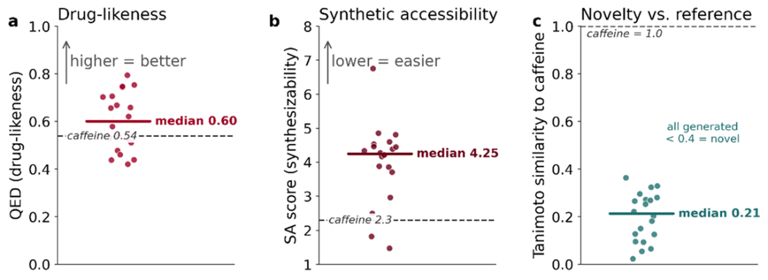
Figure I.9 QED-guided optimization seeded from caffeine, driven by the same pretrained DiffSBDD checkpoint with no retraining. The horizontal axis is the evolution generation (0 through 3) and the vertical axis is QED, where higher is more drug-like. The dark line tracks the best molecule in each generation's population, and the lighter line tracks the population mean; the dashed baseline marks caffeine's seed QED of 0.54. Over three generations (a population of 8 molecules, keeping the top 3 each round, sampled at 50 denoising steps) the best candidate climbs steadily from 0.54 to 0.72, while even the population average lifts to roughly 0.63. Each generation's children are, on average, more drug-like than their parents. We produce this result using a checkpoint that was never trained to optimize anything.
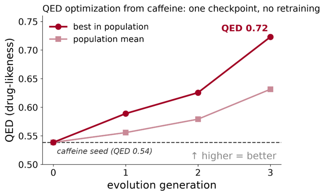
Figure I.10 Inpainting results for the caffeine purine core inside the A2A pocket. Panel (a) shows the QED of all ten generated molecules against caffeine's 0.54 baseline; the remaining panels depict six of the elaborations as 2D structures. The shared purine-derived core carried through each one, decorated with different rings, chains, and substituents, the visual signature of scaffold-hopping. This is the third distinct job we have asked a single pretrained checkpoint to do: generate freely, optimize a seed, and now elaborate a fixed scaffold.
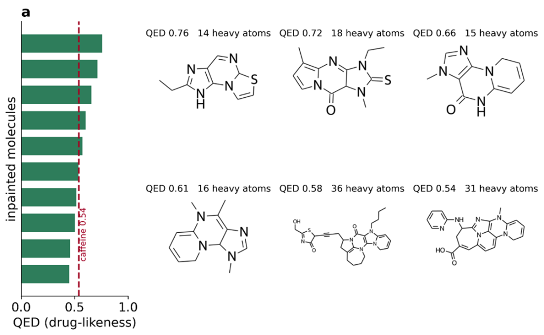
Figure I.11 The highest-QED member of our twenty generated ligands, at QED 0.79, seated inside the adenosine A2A receptor pocket from PDB 3RFM. The pocket is drawn as a translucent molecular surface, the wall of the binding site the ligand must fit against, while the generated molecule is shown as sticks with its heteroatoms picked out by color (blue nitrogen, red oxygen, yellow sulfur). The ligand nestles into the surface rather than floating outside it, placing a novel, drug-like molecule into the three-dimensional space the receptor presents.
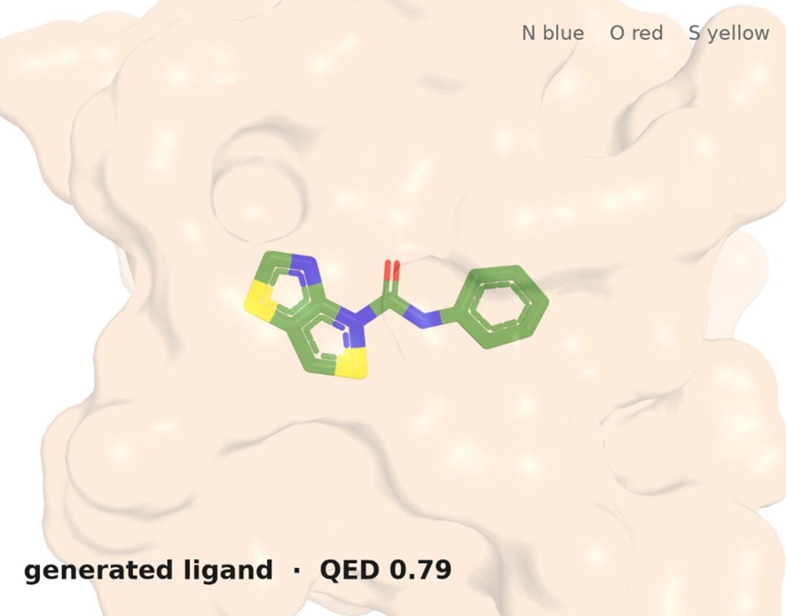
Figure I.12 Independent re-docking of the twenty pocket-conditioned ligands into the same receptor with DiffDock-L, which asks whether a second method agrees with the generator's placement. Panel (a) compares how each pose source fares on the identical PoseBusters bar, and the two fail in opposite directions: the generated poses (crimson) are good relative to the protein but strained internally, while the re-docked poses (slate) have passing internal geometry and instead violate the minimum-distance-to-protein check on more than half the ligands. Panel (b) shows the pose disagreement, with no top-ranked re-docked pose landing within 2 angstroms of its generated counterpart and only two ligands managing it among any of ten returned poses. Panel (c) pairs each ligand's distance from the co-crystal reference before and after re-docking, showing that both methods find the same site even as they disagree about the pose within it.
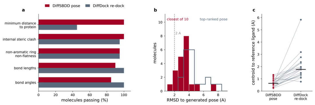
Figure I.13 The two directions of structure-based diffusion design as mirror images of a single denoising idea. On the left, DiffSBDD holds the target pocket fixed (the solid outline) and generates a new ligand inside it (the dashed output): fix the pocket, generate the ligand. On the right, all-atom RFdiffusion holds a seed ligand fixed (the solid ring) and generates a new protein pocket around it (the dashed output): fix the ligand, generate the pocket. Whichever half of the protein–ligand complex you already have, a conditioned diffusion model can be asked to design the other half to match.
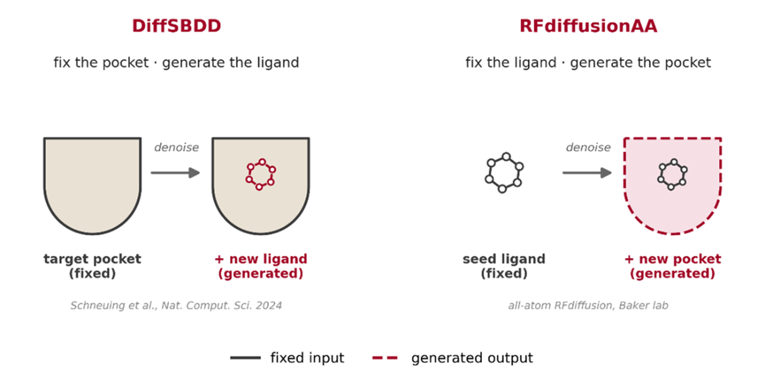
Figure I.14 Self-consistency validation of the RFdiffusion backbones. Panel (a) superimposes the three-helix-bundle backbone from RFdiffusion (red) on the ESMFold refold of its best ProteinMPNN sequence (blue), projected onto the structure's two principal axes; the two traces are nearly indistinguishable, with a Cα RMSD of 0.43 Å. Panel (b) plots the per-residue Cα deviation after superposition, which stays well below one ångström across all 80 positions (mean 0.38 Å, dashed line). Panel (c) places all 24 designs, eight sequences for each of the three backbones, in the scRMSD-versus-pLDDT plane; the green band marks the designable region (scRMSD < 2 Å, pLDDT > 70), and 23 of the 24 designs fall inside it. Panel (d) extends the test to scale, repeating the generate-design-refold loop at backbone lengths of 60, 90, 120, and 150 residues, the designable fraction holds and in fact rises from 58 percent at 60 residues to 88 percent at 150, while the median self-consistency RMSD stays below 1.5 Å throughout.
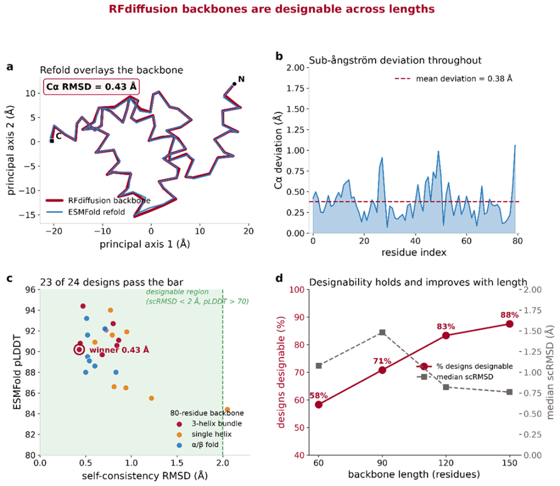
Figure I.15 The specific molecule handed from the FlowMol3 generation run of I.4 into the Boltz-2 triage step. On the left is the 2D structure, a trifluoromethoxy benzamide with SMILES Cc1ccc(NC(=O)c2ccc(OC(F)(F)F)cc2)cc1; on the right is its computed profile. It is a compact, drug-like molecule comfortably inside the size limit that Boltz-2's affinity head requires.
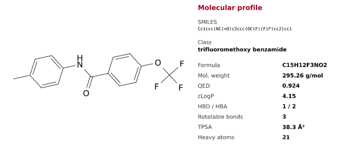
Figure I.16 Boltz-2 triage of the FlowMol3 molecule against the adenosine A2A receptor, run with the AlphaFold-DB multiple-sequence alignment. Panel (a) tracks structural confidence across five diffusion samples: ligand-interface ipTM holds around 0.95 and complex pLDDT near 0.79 (on Boltz-2's 0-to-1 scale, so about 79 out of 100), both inside the high-confidence band, so Boltz-2 is sure where the ligand sits in the pocket. Panel (b) is the affinity read: a binder probability of 0.09, well below the 0.5 call line, and a continuous value of 1.17 on the log10-IC50 scale that is not calibrated for a molecule below that line. The two panels together are the triage signal we want, a confident fold paired with a skeptical affinity, marking this drug-like-but-untargeted molecule as a weak starting point rather than a hit.
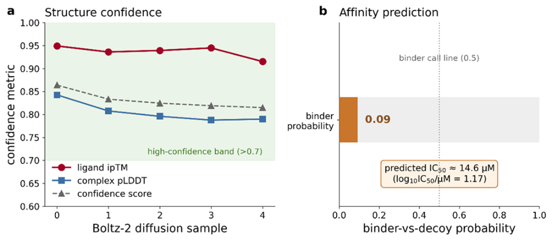
Figure I.17 Boltz-2 binder probability for seven molecules scored against the adenosine A2A target under two independent implementations: a version-pinned local build on an A100 (crimson) and NVIDIA's hosted service (slate). Panel (a) ranks the molecules, with the dashed line marking the 0.5 threshold above which the binary head calls a molecule a binder. Only caffeine, the co-crystal ligand included as a positive control, clears it under either implementation; the best pocket-conditioned design reaches 0.44 and the unconditioned FlowMol3 molecule 0.09. Panel (b) plots the two implementations against each other, with a rank correlation of 0.96 and a mean absolute difference of 0.03, so the ordering is a property of the model rather than of one build. Note that the continuous head that converts to a potency estimate is only meaningful for molecules the binary head has already called binders, and none of the generated molecules qualify.
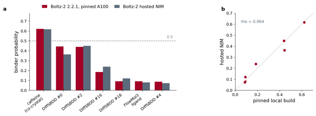
Figure I.18 The top-scoring pocket-conditioned ligand inside the adenosine A2A receptor, rendered from the Boltz-2 co-folded complex. Panel (a) shows the DiffSBDD design in crimson sticks against a gray cartoon of the receptor, with the side chains lining the pocket within 4.5 angstroms drawn in slate; this is the molecule that the highest binder probability among the five ligands scored in figure I.17, at 0.44. Panel (b) overlays Boltz-2's predicted pose for caffeine in teal after superposing the two complexes on their protein backbones. The designed molecule occupies substantially the same volume as the reference, which is what pocket conditioning is supposed to achieve and is the encouraging half of the result. The sobering half is in Figure I.17: occupying the same space as a known binder is not the same as being called one, and the affinity head clearly separates these two molecules.
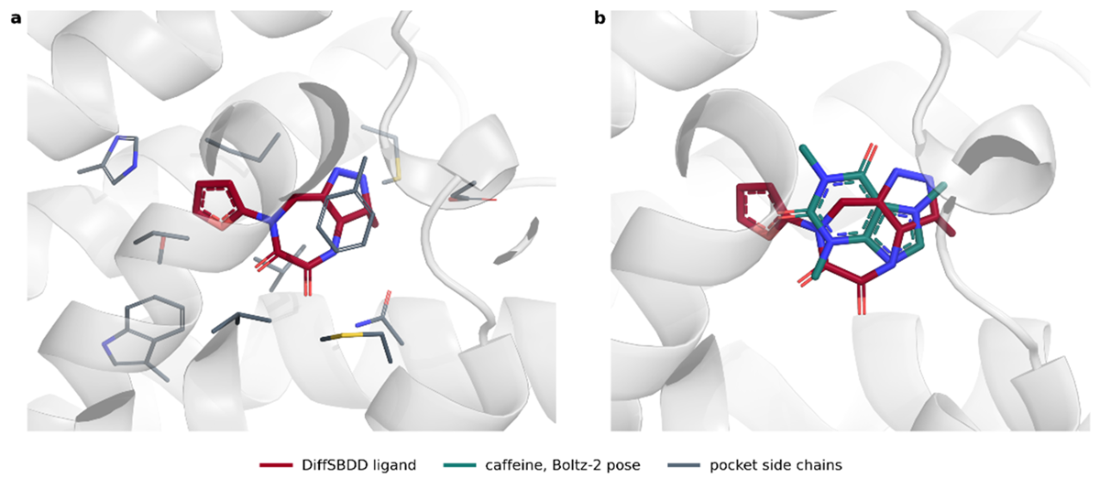
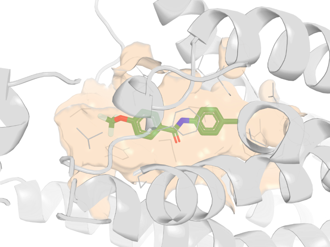
Figure I.19 The Boltz-2 co-folded complex behind the triage score. The adenosine A2A receptor is drawn as a gray cartoon with a translucent surface over the binding pocket, and the FlowMol3 trifluoromethoxy benzamide sits inside it as sticks colored by element (green carbon, blue nitrogen, red oxygen, pale-cyan fluorine). Boltz-2 is confident about where the ligand rests, even as its affinity head stays skeptical that it binds tightly.
I.8 Summary
We began this chapter with a frustration. The latent-space autoencoders of Chapter 10 and Appendix C decode a molecule in a single shot, and that one-shot leap struggles to place atoms into valid three-dimensional geometry. Diffusion and flow matching answered with a different philosophy: build the molecule gradually, by iterative refinement, so every step has only a small, learnable correction to make. First, we watched diffusion learn to reverse the arrow of noise, dissolving a target into static, then training a network to walk it back one denoising step at a time. Then we met flow matching, which replaces the stochastic reverse process with a smooth, learned velocity field: a straighter path from noise to data.
Flow matching reached the same sample quality as diffusion in far fewer sampling steps. We planted the claim on the two-moons toy, where flow matching hit target quality in about 8 steps against diffusion's 32, a roughly fourfold saving, and matched-budget comparisons were not close. Then we confirmed it on 3D molecules with FlowMol3, whose validity plateaus by around 50 sampling steps while still producing drug-like structures (a mean QED of 0.72 across the batch). At the scale of a screening campaign, requiring fewer steps is the scaling factor between designing hundreds of molecules and designing millions.
From there we turned from making molecules in a vacuum to making them for a purpose. DiffSBDD showed us pocket-conditioned design: freeze a protein binding site, sculpt a ligand to fit it, all while respecting the SE(3) symmetry that real physics obeys. Inside the adenosine A2A receptor it produced twenty valid, drug-like ligands unlike their reference, and then, from the same checkpoint and with no retraining, it optimized caffeine's drug-likeness from 0.54 to 0.72 in three short generations. We closed at the frontier, with RFdiffusion designing the protein instead of the ligand, the mirror image of DiffSBDD, and Boltz-2 standing as a triage connector that folds and scores a generated molecule to decide whether it is worth making.

 Build AI Drug Discovery Pipelines ebook for free
