Overview
Appendix E. Extended Technical Material
Figure E.1 Arbitrarily fitted examples of linear regressors for both RANSAC (left) and SVR (right).
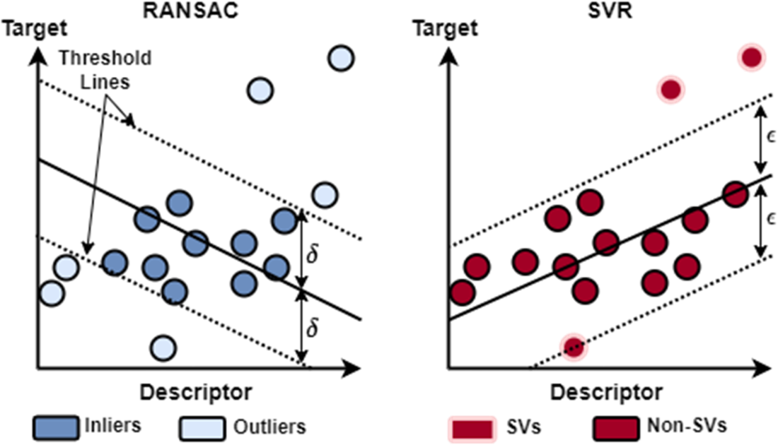
Figure E.2 Wild type EGFR in complex with LN2057 obtained by X-ray diffraction (PDB ID: pdb_00006vhn). We represent EGFR as a Gaussian surface, which renders the 3D shape of the protein in a way that emphasizes its overall volume and shape (rather than a detailed atomic structure). We color EGFR by its accessible surface area, which renders the protein surface in colors ranging from white to dark blues. The least accessible (buried) residues are colored white. The darker blues reflect greater exposure of the corresponding residues. Refer to this video on Mol* for a tutorial on visualizing biomolecular structures using Mol* in PDB.
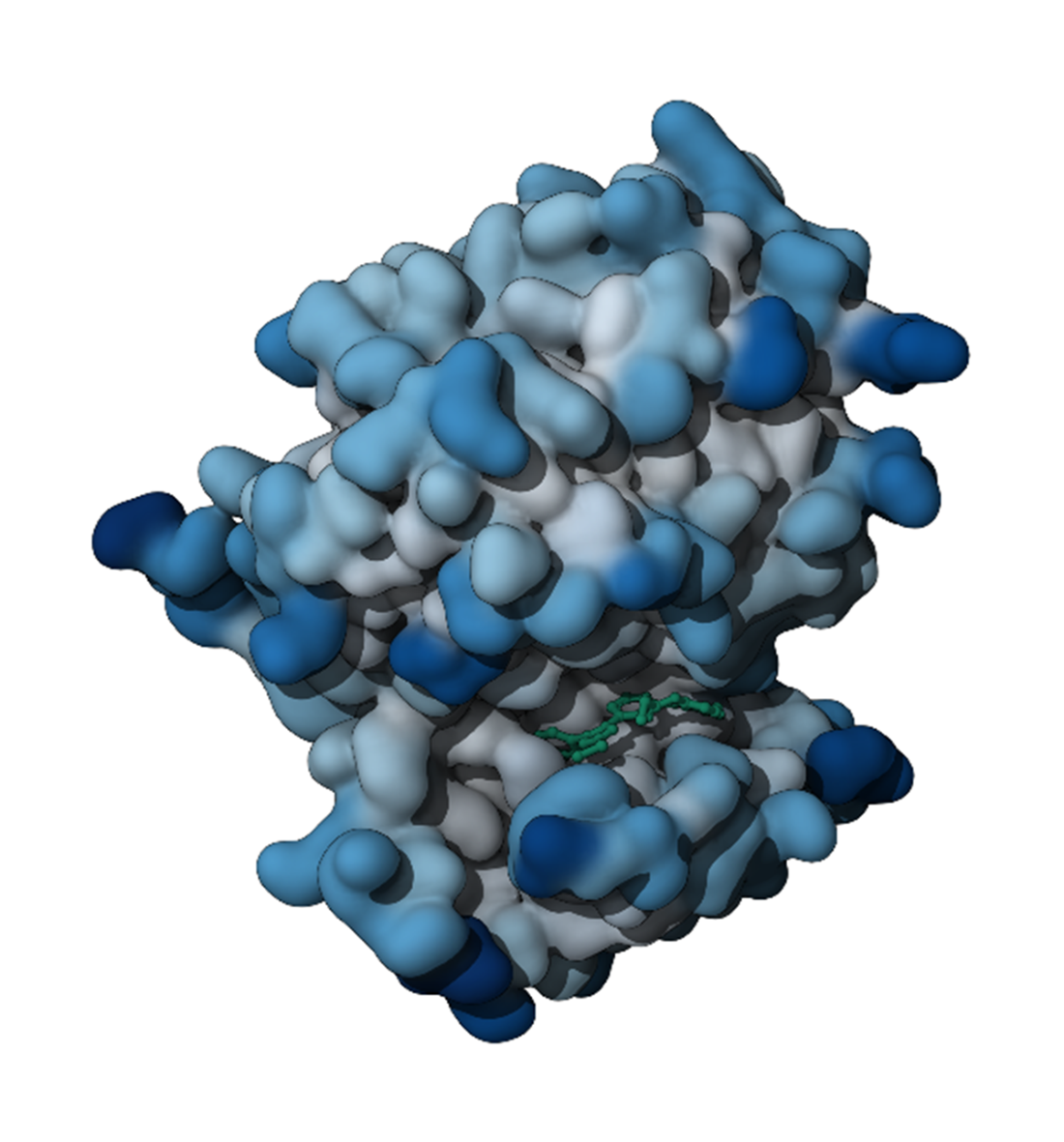
Figure E.3 An interaction map for different protein residues (y-axis) across multiple docking poses (x-axis). Each colored bar represents a specific interaction: hydrophobic interactions (green), Van der Waals contacts (gold/orange), H-bond acceptor (light blue), H-bond donor (dark blue), Pi-cation interactions (purple), and Pi-stacking interactions (magenta).
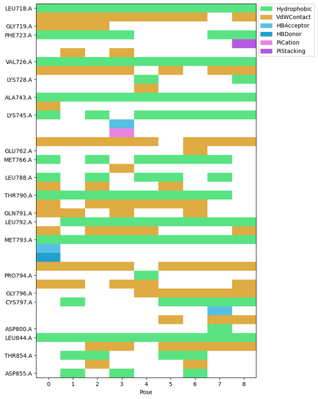
Figure E.4 2D interaction diagram displaying the ligand structure (shown in black with heteroatoms in color) and its interactions with surrounding protein residues. The residues are color-coded by their properties: aliphatic residues (green boxes), aromatic residue (purple box), basic residue (dark blue box), polar residues (cyan boxes), and sulfur-containing residues (yellow boxes). The interactions are represented by different types of dotted lines that follow the same color scheme as the interaction map.
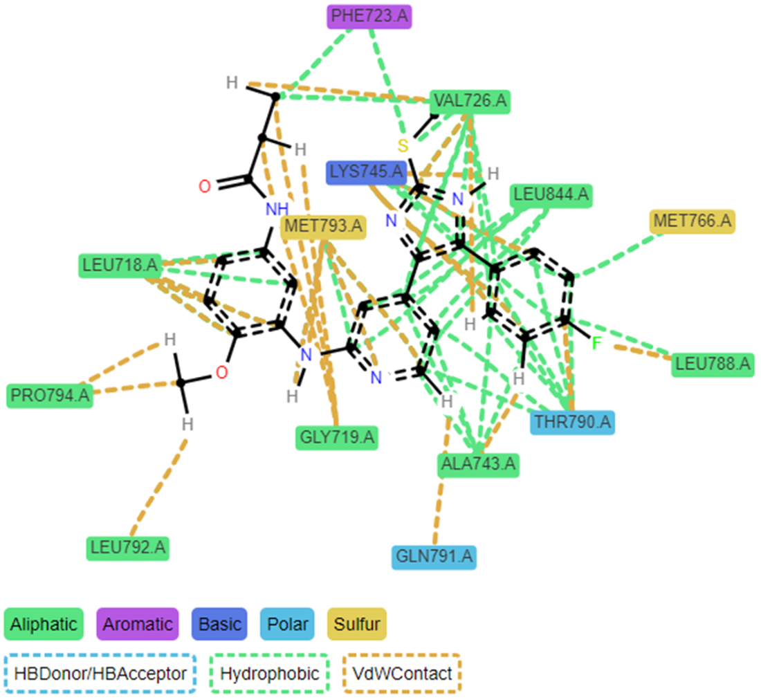
Figure E.5 3D comparison of docking poses 0 (left) and 8 (right) within the protein binding site. Both images display the protein structure as a gray ribbon with the docked ligand shown in stick form. The cyan-colored structure represents the main ligand conformation, while interacting protein residues are shown in various colors. The magenta-colored residues highlight amino acids that either have different interactions or are missing in pose 8 compared to pose 0.
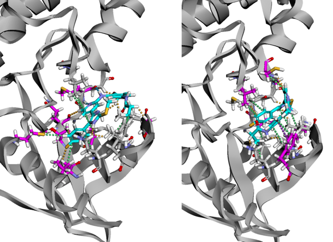
Figure E.6 The VAE modifies the standard autoencoder by introducing a probabilistic encoder that maps input molecules to probability distributions rather than single points in latent space. The encoder outputs mean (μ) and log-variance (log σ²) parameters of a Gaussian distribution. The latent vector z is sampled by combining the mean with scaled random noise (ε ~ N(0,1)). The model is trained using two loss components: reconstruction loss (measuring how well the decoder reconstructs the original molecule) and KL divergence loss (ensuring the learned distributions remain close to a standard normal distribution). This probabilistic approach creates a continuous, structured latent space where every point corresponds to a valid molecular representation, enabling reliable generation of new molecules through sampling.
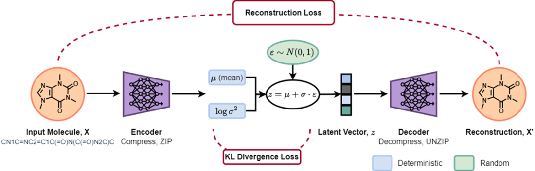
Figure E.7 Comparative latent space analysis: side-by-side scatter plots showing FDA-approved drug distributions in 2D latent spaces, with each USAN stem class in a different color]
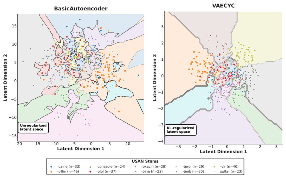
Figure E.8 Latent Space Interpolation. We illustrate a smooth transition between two molecules within the VAE-CYC's 2D latent space. The space is colored by the Natural Product-likeness Score. The path begins at a "Start" molecule and moves linearly to an "End" molecule, with decoded intermediates shown at numbered steps. The properties of the generated molecules, including Tanimoto similarity to the start/end points and the Natural Product-likeness Score, change gradually along the path, demonstrating the continuity and organizational quality of the latent space.
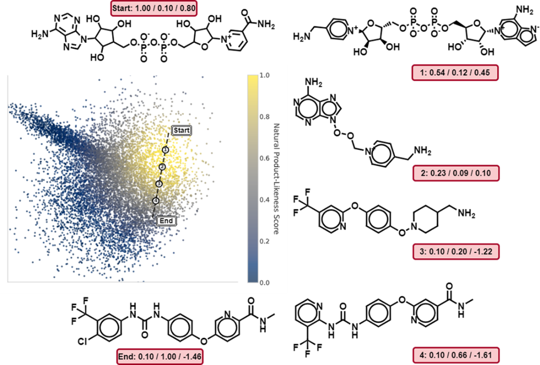
Figure E.9 Continuity of the VAE-CYC Latent Space Under Noise Perturbation. The plot shows the average Tanimoto similarity between a set of starting molecules and the molecules generated after successively applying steps of Gaussian noise to their latent vectors. The three curves correspond to different noise magnitudes (standard deviation σ). The gradual decrease in similarity, especially for smaller noise levels (σ=0.1), demonstrates that the latent space is smooth and continuous, where small perturbations to a latent vector result in small changes to the decoded molecular structure.
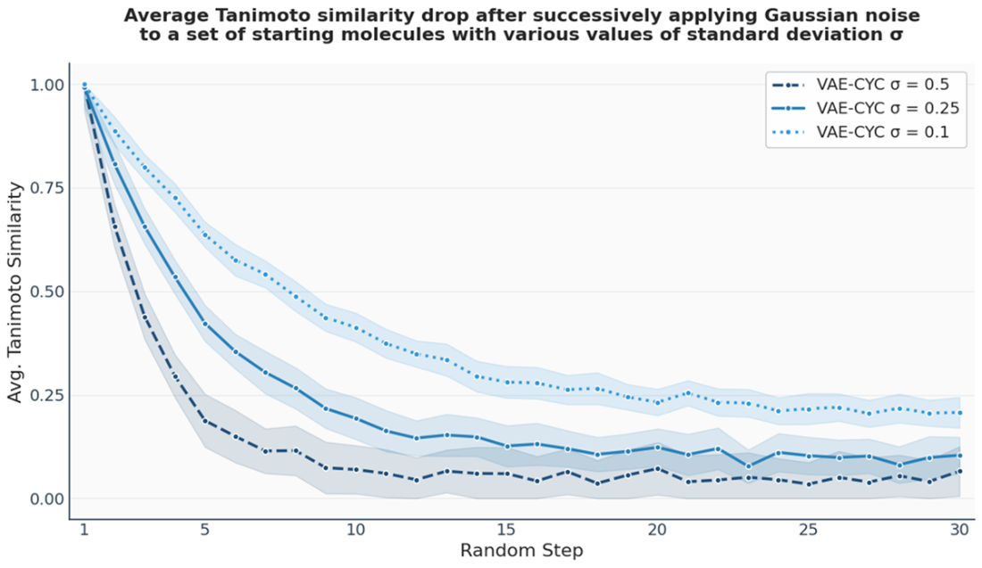
Figure E.10 GNN Node Embedding Process. A GNN functions as an encoder that maps nodes from a graph (left) into a low-dimensional, continuous embedding space (right). For each node, such as 'W' and 'S', the GNN processes its features and the structure of its local neighborhood to generate a corresponding embedding vector. The objective is to learn a mapping where the geometric relationships between these vectors in the embedding space capture the structural relationships and similarities of the nodes in the original graph.
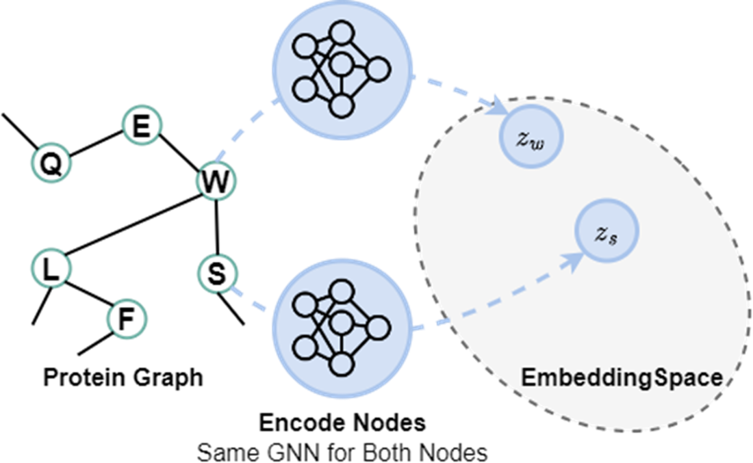
Figure E.11 The Message Passing Mechanism in Graph Neural Networks. A node updates its feature vector (or embedding) by incorporating information from its local neighborhood. The resultant aggregate and update operations are carried out across every node at once for the current layer, and also across further rollouts across additional layers. Each GNN layer shares the same weights. At the end, the final node embeddings are pooled to provide a graph-level embedding for our drug-target affinity prediction task. This process is carried out separately across the molecule branch and the protein branch of DGraphDTA.
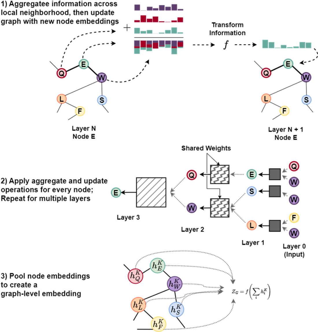
Figure E.12 Visualization of multi-head attention weights for the Caffeine molecule in a GAT. The four heads in Layer 1 learn to focus on different atomic relationships, as shown by the varying attention weights (color intensity) on the directed edges connecting the atoms. Each head specializes in capturing distinct structural patterns; for instance, one head might prioritize a carbonyl group, while another emphasizes the nitrogen atoms in a specific ring. This specialization allows the model to capture diverse chemical features in parallel.
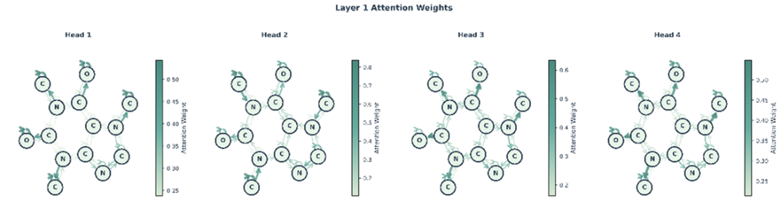
Figure E.13 The outputs from Layer 1 in figure E.12 are aggregated by Layer 2, which learns a new attention distribution based on the features extracted by the first layer, creating a richer representation for downstream tasks. Layer 2 similarly has multiple heads (we show only one head for brevity).
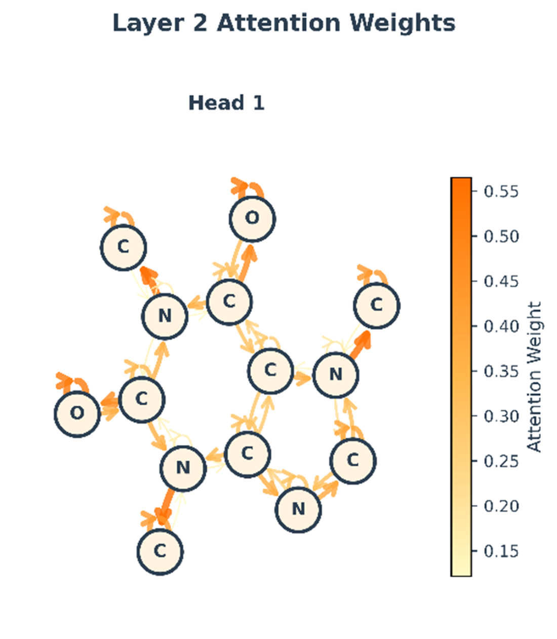
Figure E.14 Illustration of the Message-Passing Mechanism with Edge-Conditions and Directionality. The following visual shows how we can extend message passing framework to accommodate edge-conditioned features, directionality of message passing, and residual connections. A sample graph is shown, centered on the target node (black), which is connected to its neighboring nodes, providing an example information flow for the 2-layer unidirectional MPNN. At each graph convolution layer, node u is influenced by messages from its parents node(s), NP, and influences its child node(s), NC. Messages are conditioned by edge information. For each message passing iterations, the edge features remain constant but are parameterized by distinct MLPs. Output embeddings from each layer are concatenated and fed through another MLP to produce class predictions. Node u is only exposed to, at most, information from the dark grey nodes and is disconnected from half of the network. A residual connection (blue arrow) adds the node's representation from the first iteration to the result of the second. Finally, the updated representation is passed through a final output MLP to generate a prediction, such as the class probabilities [0.8, 0.2].
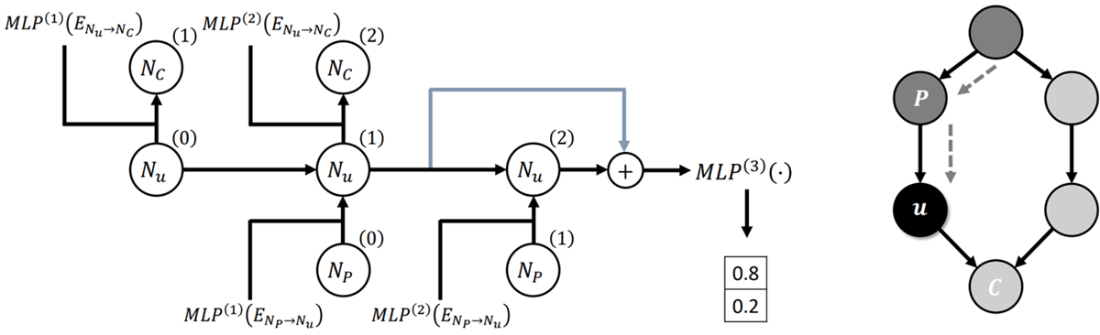
Figure E.15 Flow matching visualized in the protein structure prediction setting. (A) The biological folding process transforms an unfolded chain (t=0) into a folded structure (t=1). (B) The computational flow matching process mimics this by learning a velocity field that guides a distribution of random noise (source) to match the distribution of real protein structures (target) over a virtual timeline.
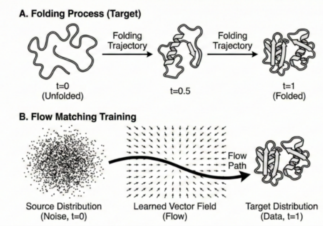
Figure E.16 (Left) A SimpleFold prediction for target sequence 7ftv_A. The structure is colored by predicted confidence (pLDDT), ranging from red (low confidence) to blue (high confidence). The pervasive blue coloring indicates that the model has high certainty in the predicted backbone geometry. (Right) An all-atom rendering of the predicted structure from Figure E.16. While ribbon diagrams show the backbone path, this visualization includes all side-chain atoms, allowing researchers to inspect atomic packing density and specific chemical interactions within the protein core.
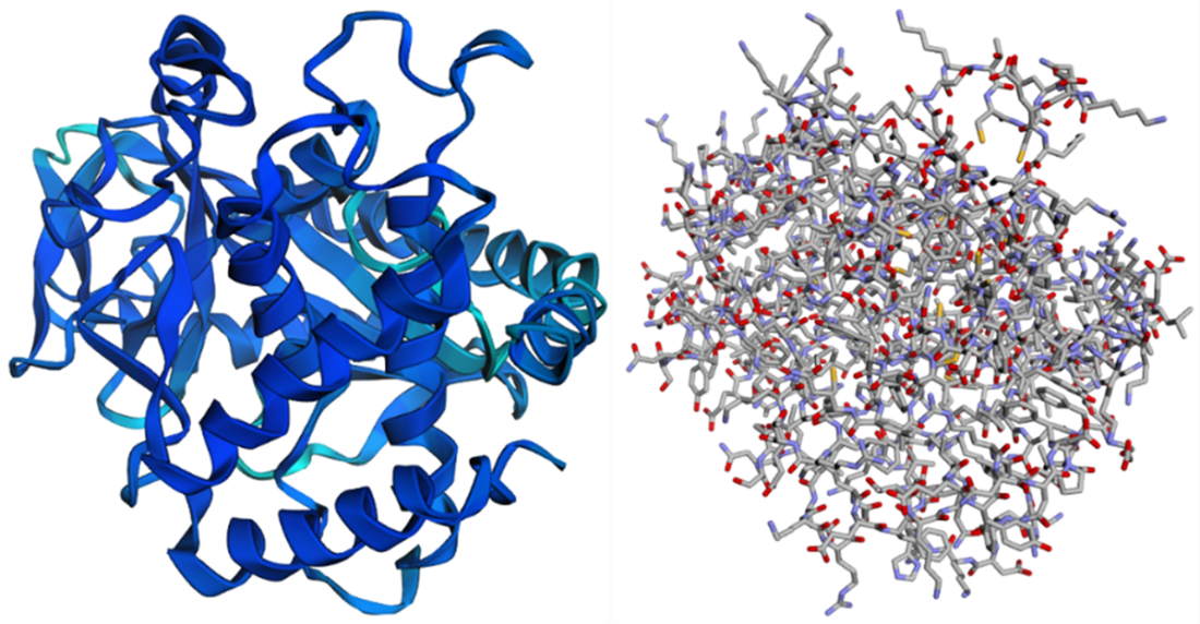
Figure E.17 Confidence vs. Deviation Analysis for protein 7ftv_A. The blue line tracks the predicted confidence (pLDDT), while the orange line tracks the actual Cα deviation (in Angstroms) from the ground truth. Note the inverse relationship: regions with high pLDDT (e.g., residues 150-350) exhibit very low deviation (< 1 Angstrom), corresponding to the stable hydrophobic core. Conversely, sharp drops in confidence (residues ~50 and ~200) correlate with spikes in deviation, indicating flexible loops or disordered regions where the model identifies its own uncertainty.
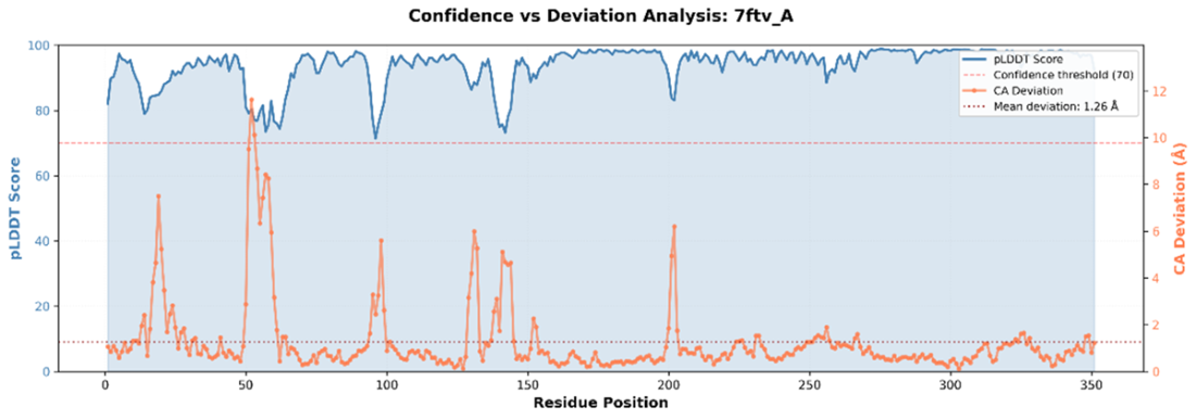
Figure E.18 Structural alignment of the prediction (red) against experimental ground truth (blue). Visuals complement numerical metrics like TM-score (0.949) and RMSD (2.015), showing near-perfect agreement in the core helices with slight deviations in flexible loop regions. We can see which regions align or diverge, whether the overall fold is correct, and how significant errors are in context of the full structure.
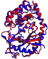
Figure E.19 Top row (distance matrices): The Ground Truth (left) and Predicted (center) matrices show the pairwise distance between all residues, where yellow indicates proximity and blue indicates separation. The Difference map (right) highlights errors: dark red bands indicate regions (e.g., around residue 50) where the predicted distances deviate significantly (> 5 Angstroms) from the experimental structure. Bottom Row (Contact Maps): Binary maps showing residue pairs within 8 Angstroms. The Difference map (right) plots false positives (blue) and false negatives (red). This view confirms that while the global fold is largely correct (diagonal consistency), the model struggles to capture specific long-range contacts in the flexible loop regions.
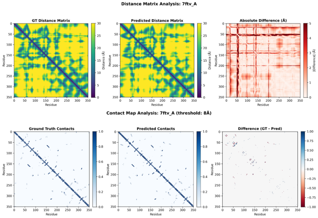
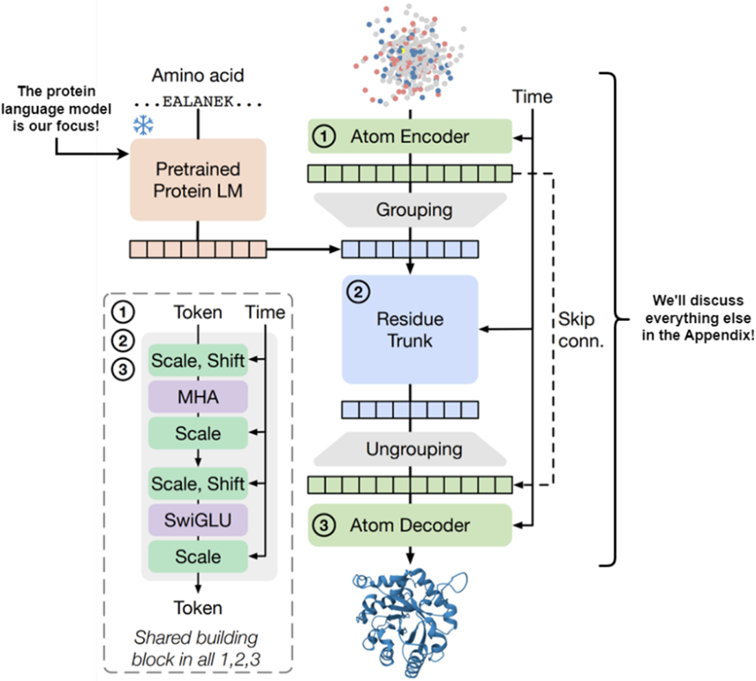
Figure E.20 SimpleFold splits into a PLM (left) that extracts sequence features, and a structure generation module (right) involving an Atom Encoder and Residue Trunk. This chapter focuses on the PLM.

 Build AI Drug Discovery Pipelines ebook for free
