3 Classify images with a vision transformer (ViT)
This chapter introduces how to repurpose transformers for vision by treating images as sequences, bridging your understanding from text models to image tasks. It explains the core ViT idea: split an image into fixed-size patches that become tokens, add a special classification token, and use self-attention to capture both local details and long-range dependencies. Framed as a key step in a broader text-to-image roadmap, the chapter focuses on image classification to build intuition and skills that generalize to more advanced generative applications later.
Concretely, 32x32 RGB images from CIFAR-10 are divided into an 8x8 grid (64 patches). Each patch is projected to a 48-dimensional token embedding (via a convolution with kernel and stride equal to the patch size), the CLS token is prepended, and learned positional encodings of the same dimensionality are added, yielding a 65x48 input sequence per image. The model is an encoder-only ViT with four stacked transformer blocks, each combining multi-head self-attention (four heads) and a GELU-activated feed-forward network (48→192→48), wrapped with layer normalization and residual connections. A linear classification head reads the CLS representation to produce logits over the ten classes, and the implementation can expose attention maps for interpretability.
The training pipeline prepares CIFAR-10 with normalization and simple augmentations, uses batched data loaders, and optimizes with AdamW and cross-entropy loss, leveraging automatic mixed precision for speed. Early stopping on test loss (with patience) selects the best checkpoint and limits overfitting; in the reference run, the model achieves around 56% accuracy—well above chance—while attention visualizations reveal which image regions drive decisions by aggregating CLS-to-patch attention across heads and layers and upscaling to image resolution. The chapter closes by noting practical ways to improve accuracy (e.g., training longer) and sets the stage for an encoder–decoder setup that generates image captions in the next chapter.
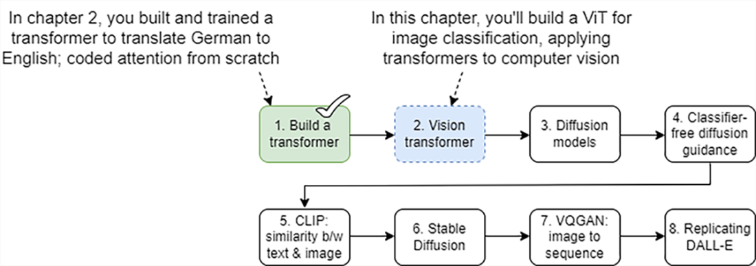
The eight-step roadmap for building a text-to-image generator from scratch. In this chapter, you’ll focus on step 2: building a vision transformer (ViT) for image classification. This is your bridge from transformers for text to transformers for images, showing how to represent visual information as sequences of tokens. This is an essential concept for subsequent chapters.
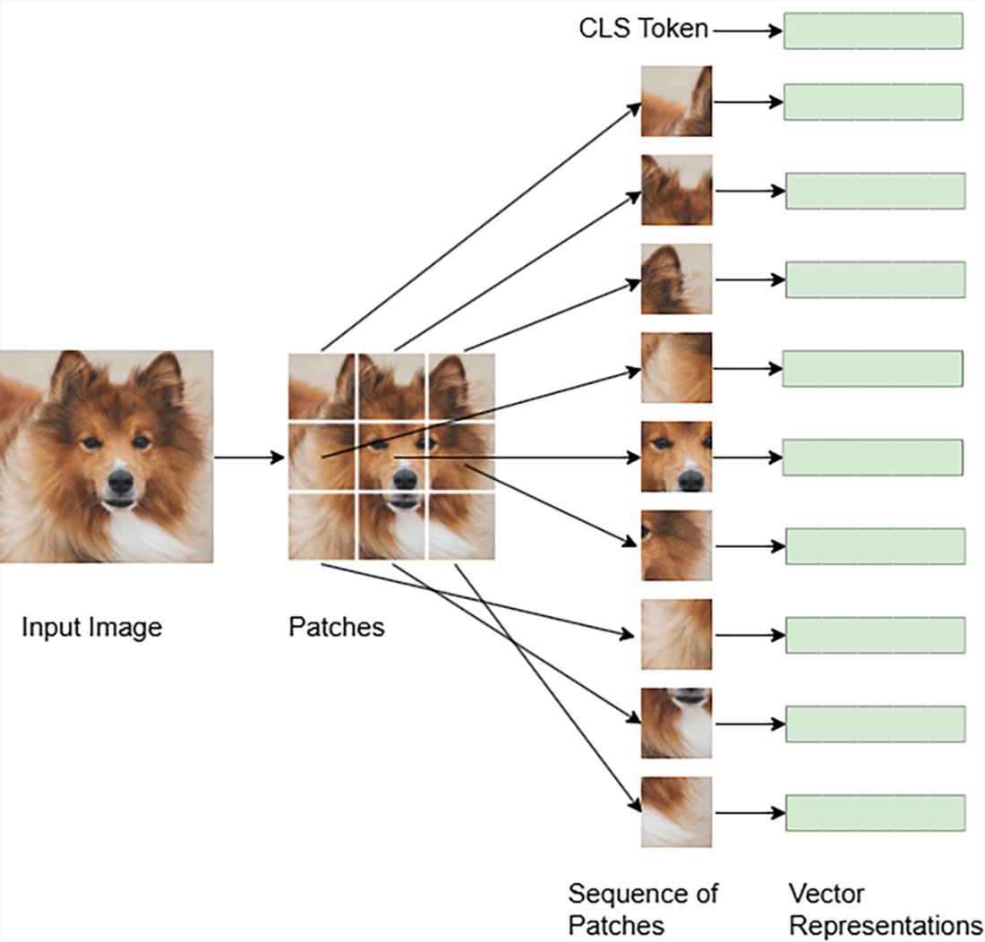
To convert an image into a sequence, the image is first divided into fixed-size patches. The patches are ordered into a sequence: top left patch first, then the patch to the right, …, and finally the bottom right patch. We often add a class token at the beginning of the sequence, which is used to aggregate information in the whole sequence. Each image patch is converted into a vector (token embedding).
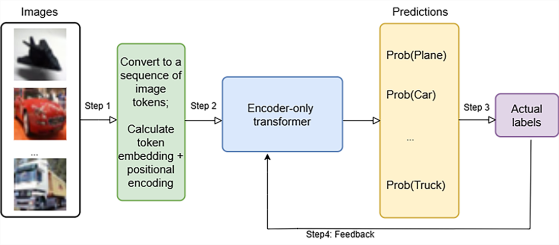
The steps involved in training a vision transformer to classify images. We’ll use the (image, label) pairs in the CIFAR-10 dataset to train the model. Images are first converted to sequences of image tokens. We then calculate the token embeddings and positional encodings of elements in the sequence. The sum of token embeddings and positional encodings is the input embeddings, which are then fed to an encoder-only transformer. The transformer predicts the label of each image. We then compare the prediction with the actual labels and calculate the cross-entropy loss. We tweak the model parameters to minimize this loss.
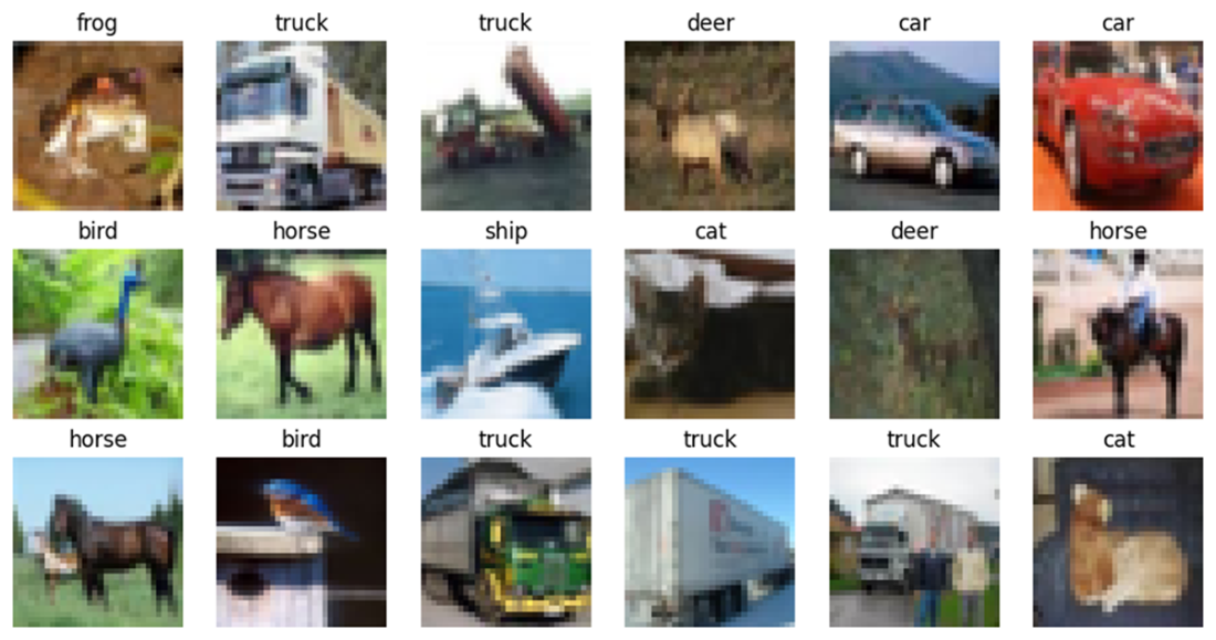
Sample images from the CIFAR-10 dataset. The dataset contains ten classes of color images: plane, car, bird, …, and truck. Each image has a dimension of 3x32x32: three color channels (red, green, blue) with a height and width of 32 pixels. The class label is on top of each image.
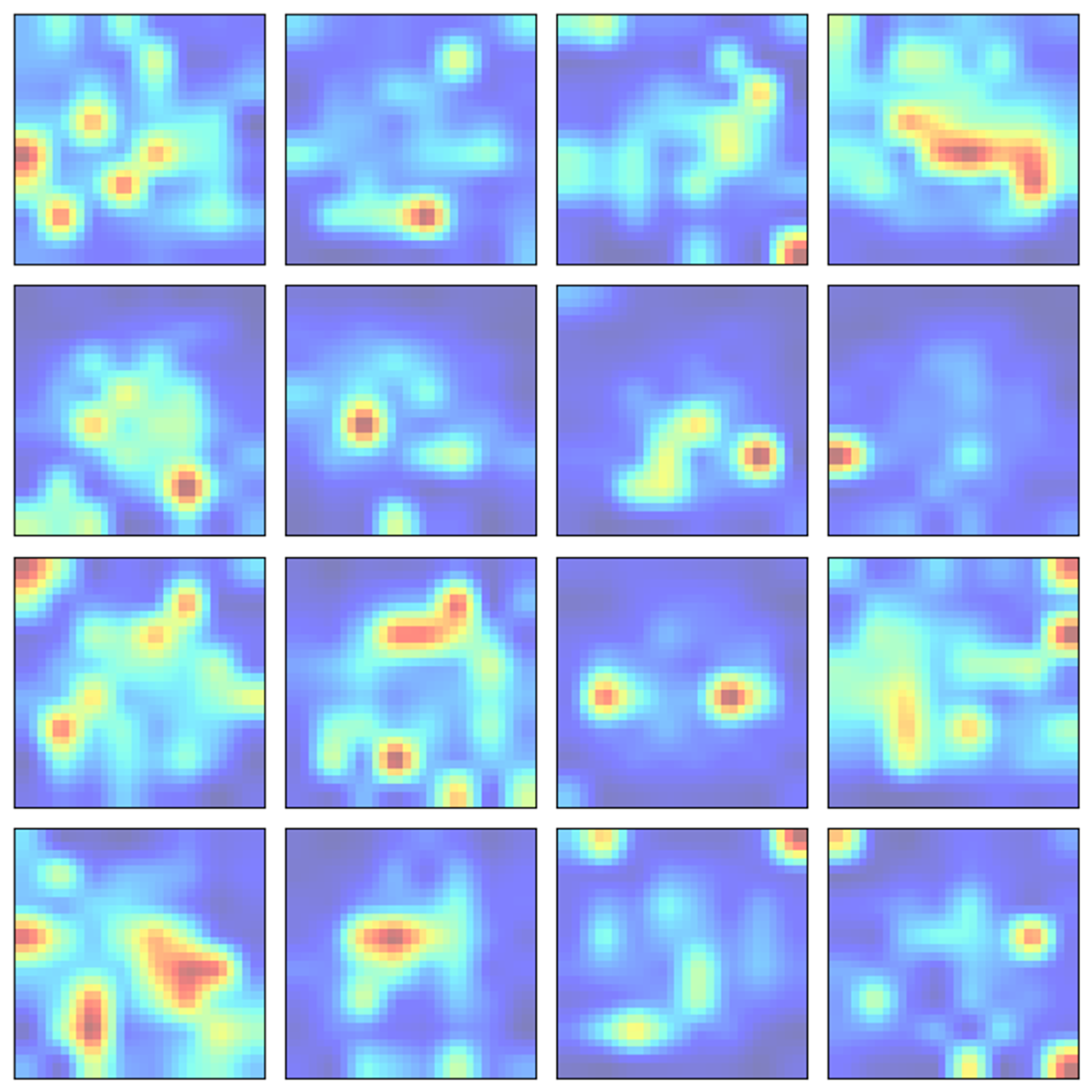
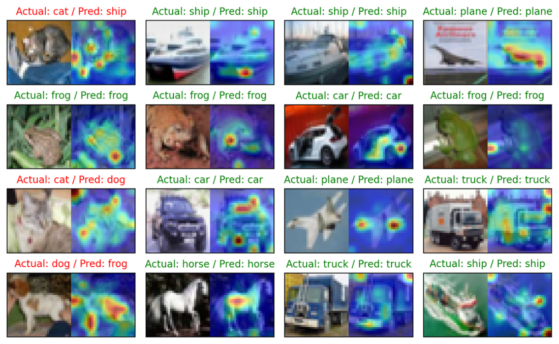
The attention maps for 16 test images. For each image, we first extract and concatenate the attention maps from the four encoder layers into one tensor. Then, we isolate the maps representing the attention between the CLS token and the 64 image patches. Averaging the attention maps across the four heads and four encoder layers yields a tensor of 64 values per image. These values are reshaped into an 8×8 grid and then upscaled to 32×32 to match the original image size. Finally, the attention maps for the 16 images are displayed in a 4×4 grid.
Make predictions on CIFAR-10 images using the trained ViT classifier. In each pair, the left image is the original image from CIFAR-10 and the right image is the attention map generated by the trained ViT. On top of each pair of images, we print out the actual label and the predicted label.
Summary
- In transformer-based text-to-image generation, a crucial step is transforming an image into a token sequence, much like converting text into a sequence of words.
- A ViT processes an image by dividing it into fixed-size patches and treating each patch as a token. These patches are then ordered sequentially. The sequence starts with the top-left patch, followed by the patch to the right in the same row, ending with the bottom-right patch. To facilitate tasks like image classification, a special class token CLS is added at the beginning of the sequence.
- Image tokens, including the class token at the beginning of the sequence, are embedded into a vector through a process known as image embedding. Transformers and their self-attention mechanism do not account for the order of inputs. To address this, we add positional encodings to the token embeddings. These encodings inject information about the relative positions of patches within the image, enabling the model to understand spatial structure.
- Fixed positional encodings are predefined, deterministic values added to the input embeddings. These encodings are static and do not change during training. On the other hand, learned positional encodings are model parameters that are updated during training, much like the weights in a neural network. This allows the model to discover the optimal positional encodings for a given task and dataset.
- A trained ViT can be used to classify images. The attention mechanism in ViT can also show the attention map the trained model pays to various parts of an image.
FAQ
What is a Vision Transformer (ViT) and why use it for images?
ViT applies the transformer architecture, originally built for sequences like text, to images by splitting an image into fixed-size patches and treating each patch as a token. This lets the model use self-attention to capture both local and long-range relationships across an image, enabling strong performance on classification and other vision tasks.How do you convert a CIFAR-10 image into a token sequence?
- Start with a 3x32x32 RGB image.- Divide it into an 8x8 grid of patches (patch size 4x4), producing 64 patches.
- Project each patch to a 48-dimensional vector (token embedding).
- Prepend a CLS token to the sequence for classification, making 65 tokens in total.
- Add learned positional encodings (also 48-d) to each token. Final input shape per image: (65, 48).
What is the CLS token and how is it used?
The CLS (classification) token is a learned vector prepended to the sequence of patch tokens. It is not tied to a specific image patch; instead, it aggregates information from the entire sequence through self-attention. At the output of the encoder, the CLS token’s representation is passed to a linear layer to produce logits for the target classes.Why are positional encodings needed, and why use learned positional encodings here?
Self-attention is permutation-invariant and doesn’t know token order by itself. Positional encodings inject spatial order so the model can reason about patch locations. This chapter uses learned positional encodings (size 65x48 for CIFAR-10) so the model can adapt position information to the dataset’s non-uniform spatial relationships. Fixed encodings are parameter-free and extrapolate to longer sequences, but learned encodings can be more flexible and performant for images.How are patch embeddings computed in this ViT?
A Conv2d layer with kernel_size=stride=patch_size (4) maps non-overlapping 4x4 patches into 48 channels. For a 3x32x32 image, the Conv2d output is 48x8x8, which is then flattened to a sequence of 64 tokens of dimension 48 (shape 64x48 per image).How does multi-head self-attention work in this model?
Token embeddings are linearly projected into queries, keys, and values. With hidden size 48 and 4 heads, each head operates on 12-d subspaces. Scaled dot-product attention computes attention scores (Q·Kᵀ/√dₖ), applies softmax to get attention weights, and uses them to combine values. Attention maps per layer have shape [batch, heads, seq_len, seq_len] = [32, 4, 65, 65] in the example.What is inside an encoder block and why use residual connections and layer normalization?
Each block has: (1) multi-head self-attention, (2) a position-wise MLP with GELU activation (48 → 192 → 48), plus pre-layer normalization and residual connections around both sublayers. Residuals stabilize training and mitigate vanishing gradients; layer norm improves optimization by normalizing activations.How is the ViT turned into an image classifier?
The encoder-only ViT (4 stacked encoder blocks) processes the token sequence. The output for the CLS token (position 0) is fed into a linear classification head producing 10 logits (for CIFAR-10). Predictions are obtained by applying softmax (for probabilities) or argmax (for class labels).How is the model trained in this chapter?
- Dataset: CIFAR-10 (3x32x32), with standard transforms and simple augmentations (e.g., random flip/crop) for training.- Batching: 32 images; shuffle for training.
- Loss: Cross-entropy.
- Optimizer: AdamW with lr=0.01 and weight_decay=1e-2.
- Speedup: PyTorch automatic mixed precision (torch.amp GradScaler and autocast).
- Early stopping: Stop if test loss doesn’t improve for 3 epochs (best weights saved). Training ran up to 100 epochs with early stop around epoch 13 in the example.
How do you visualize what the ViT attends to?
- Collect attention maps from all 4 encoder layers and 4 heads → concatenate to [batch, 16, 65, 65].- Extract attention from CLS to the 64 patch tokens (index 0 to 1:), yielding [batch, 16, 64].
- Average across heads/layers → [batch, 64], reshape to 8x8, then upsample to 32x32.
- Overlay the heatmap on the original image to see which regions influenced the prediction. Each column of an attention matrix sums to 1, forming a valid attention distribution.

 Build a Text-to-Image Generator (from Scratch) ebook for free
