3 Coding Attention Mechanisms

This chapter builds a bridge from tokenized, embedded text to the core computation that powers modern LLMs: attention. It motivates attention by highlighting the bottleneck of pre‑transformer encoder–decoder RNNs, which tried to compress an entire input into a single hidden state and struggled with long‑range dependencies. The chapter’s roadmap incrementally codes four attention variants—starting from a minimal, weight‑free self‑attention, then adding trainable projections for scaled dot‑product attention, introducing causal masking for autoregressive generation, and finally assembling multi‑head attention—culminating in a compact, efficient module ready to slot into a GPT‑style architecture.

The narrative first demystifies self‑attention as a way to build context vectors for each token by weighting all tokens in the sequence according to pairwise similarity. It shows how to compute attention scores via dot products and normalize them with softmax so weights sum to one, then generalizes this to compute all tokens’ context vectors efficiently with matrix operations. Next, it upgrades to the practical, learnable version—scaled dot‑product attention—by projecting embeddings into queries, keys, and values with trainable matrices, scaling scores by the square root of the key dimension to stabilize gradients, and packaging the operations into concise PyTorch classes that support batched inputs.

To make attention usable for next‑token prediction, the chapter adds causal masking so each position can only attend to itself and prior tokens, implementing the mask efficiently by inserting negative infinities before softmax. It further regularizes training by applying dropout to attention weights. The final step is multi‑head attention: first illustrated by stacking several causal attention modules and concatenating their outputs, then implemented efficiently by splitting the projected Q/K/V across heads with reshaping and transposition, performing batched head‑wise matmuls, and fusing outputs with an optional projection layer. The result is an attention module that can attend to multiple representational subspaces in parallel and is ready for integration into the full LLM in the following chapter.

A mental model of the three main stages of coding an LLM, pretraining the LLM on a general text dataset, and finetuning it on a labeled dataset. This chapter focuses on attention mechanisms, which are an integral part of an LLM architecture.

The figure depicts different attention mechanisms we will code in this chapter, starting with a simplified version of self-attention before adding the trainable weights. The causal attention mechanism adds a mask to self-attention that allows the LLM to generate one word at a time. Finally, multi-head attention organizes the attention mechanism into multiple heads, allowing the model to capture various aspects of the input data in parallel.

When translating text from one language to another, such as German to English, it's not possible to merely translate word by word. Instead, the translation process requires contextual understanding and grammar alignment.

Before the advent of transformer models, encoder-decoder RNNs were a popular choice for machine translation. The encoder takes a sequence of tokens from the source language as input, where a hidden state (an intermediate neural network layer) of the encoder encodes a compressed representation of the entire input sequence. Then, the decoder uses its current hidden state to begin the translation, token by token.

Using an attention mechanism, the text-generating decoder part of the network can access all input tokens selectively. This means that some input tokens are more important than others for generating a given output token. The importance is determined by the so-called attention weights, which we will compute later. Note that this figure shows the general idea behind attention and does not depict the exact implementation of the Bahdanau mechanism, which is an RNN method outside this book's scope.

Self-attention is a mechanism in transformers that is used to compute more efficient input representations by allowing each position in a sequence to interact with and weigh the importance of all other positions within the same sequence. In this chapter, we will code this self-attention mechanism from the ground up before we code the remaining parts of the GPT-like LLM in the following chapter.

The goal of self-attention is to compute a context vector, for each input element, that combines information from all other input elements. In the example depicted in this figure, we compute the context vector z(2). The importance or contribution of each input element for computing z(2) is determined by the attention weights α21 to α2T. When computing z(2), the attention weights are calculated with respect to input element x(2) and all other inputs. The exact computation of these attention weights is discussed later in this section.

The overall goal of this section is to illustrate the computation of the context vector z(2) using the second input element, x(2) as a query. This figure shows the first intermediate step, computing the attention scores ω between the query x(2) and all other input elements as a dot product. (Note that the numbers in the figure are truncated to one digit after the decimal point to reduce visual clutter.)

After computing the attention scores ω21 to ω2T with respect to the input query x(2), the next step is to obtain the attention weights α21 to α2T by normalizing the attention scores.

The final step, after calculating and normalizing the attention scores to obtain the attention weights for query x(2), is to compute the context vector z(2). This context vector is a combination of all input vectors x(1) to x(T) weighted by the attention weights.

The highlighted row shows the attention weights for the second input element as a query, as we computed in the previous section. This section generalizes the computation to obtain all other attention weights.

In self-attention, we begin by computing the attention scores, which are then normalized to obtain attention weights that sum up to 1. These attention weights are used to compute the context vectors as a weighted sum of the inputs.

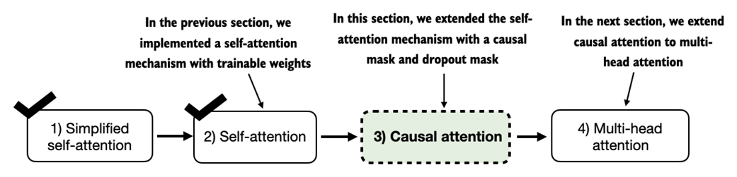
A mental model illustrating how the self-attention mechanism we code in this section fits into the broader context of this book and chapter. In the previous section, we coded a simplified attention mechanism to understand the basic mechanism behind attention mechanisms. In this section, we add trainable weights to this attention mechanism. In the upcoming sections, we will then extend this self-attention mechanism by adding a causal mask and multiple heads.

In the first step of the self-attention mechanism with trainable weight matrices, we compute query (q), key (k), and value (v) vectors for input elements x. Similar to previous sections, we designate the second input, x(2), as the query input. The query vector q(2) is obtained via matrix multiplication between the input x(2) and the weight matrix Wq. Similarly, we obtain the key and value vectors via matrix multiplication involving the weight matrices Wk and Wv.

The attention score computation is a dot-product computation similar to what we have used in the simplified self-attention mechanism in section 3.3. The new aspect here is that we are not directly computing the dot-product between the input elements but using the query and key obtained by transforming the inputs via the respective weight matrices.

After computing the attention scores ω, the next step is to normalize these scores using the softmax function to obtain the attention weights α.

In the final step of the self-attention computation, we compute the context vector by combining all value vectors via the attention weights.

In self-attention, we transform the input vectors in the input matrix X with the three weight matrices, Wq, Wk, and Wv. Then, we compute the attention weight matrix based on the resulting queries (Q) and keys (K). Using the attention weights and values (V), we then compute the context vectors (Z). (For visual clarity, we focus on a single input text with n tokens in this figure, not a batch of multiple inputs. Consequently, the 3D input tensor is simplified to a 2D matrix in this context. This approach allows for a more straightforward visualization and understanding of the processes involved. Also, for consistency with later figures, the values in the attention matrix do not depict the real attention weights.)

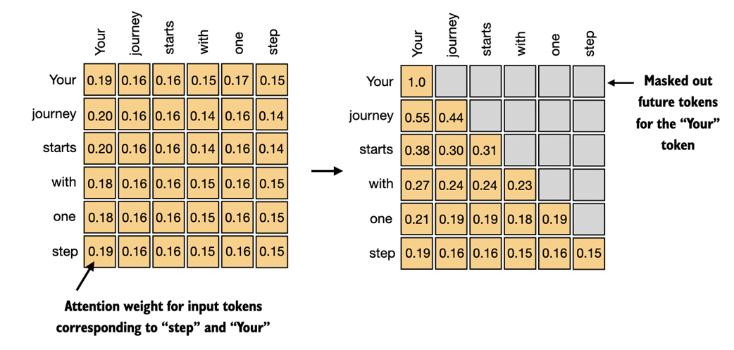
In causal attention, we mask out the attention weights above the diagonal such that for a given input, the LLM can't access future tokens when computing the context vectors using the attention weights. For example, for the word "journey" in the second row, we only keep the attention weights for the words before ("Your") and in the current position ("journey").

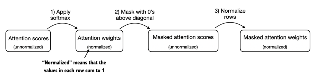
One way to obtain the masked attention weight matrix in causal attention is to apply the softmax function to the attention scores, zeroing out the elements above the diagonal and normalizing the resulting matrix.

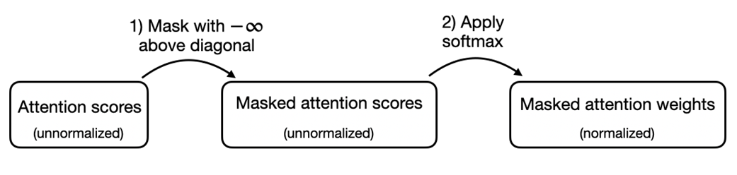
A more efficient way to obtain the masked attention weight matrix in causal attention is to mask the attention scores with negative infinity values before applying the softmax function.

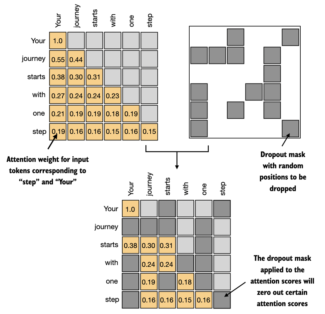
Using the causal attention mask (upper left), we apply an additional dropout mask (upper right) to zero out additional attention weights to reduce overfitting during training.

A mental model summarizing the four different attention modules we are coding in this chapter. We began with a simplified attention mechanism, added trainable weights, and then added a casual attention mask. In the remainder of this chapter, we will extend the causal attention mechanism and code multi-head attention, which is the final module we will use in the LLM implementation in the next chapter.

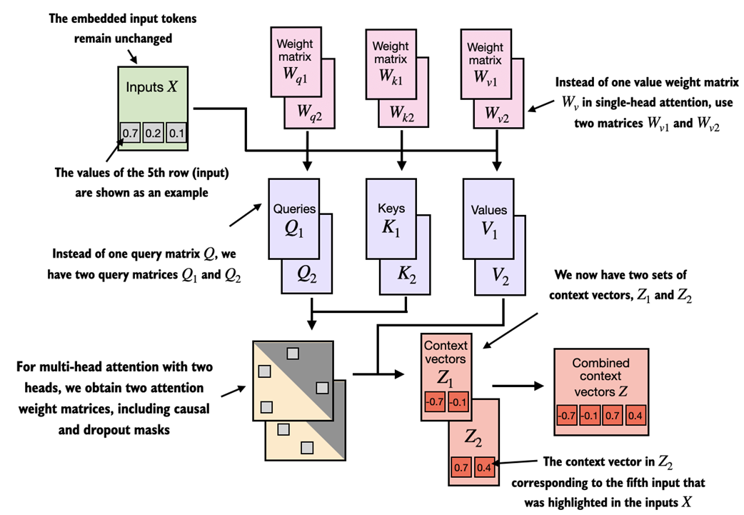
The multi-head attention module in this figure depicts two single-head attention modules stacked on top of each other. So, instead of using a single matrix Wv for computing the value matrices, in a multi-head attention module with two heads, we now have two value weight matrices: Wv1 and Wv2. The same applies to the other weight matrices, Wq and Wk. We obtain two sets of context vectors Z1 and Z2 that we can combine into a single context vector matrix Z.

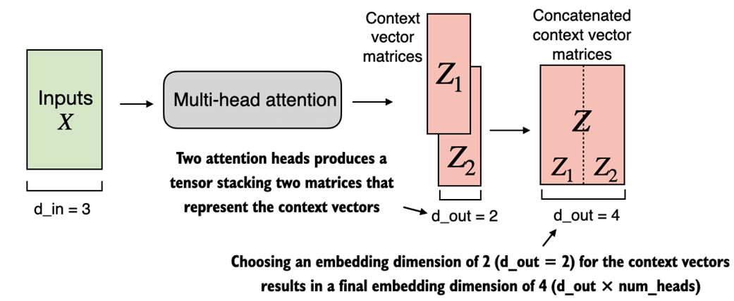
Using the MultiHeadAttentionWrapper, we specified the number of attention heads (num_heads). If we set num_heads=2, as shown in this figure, we obtain a tensor with two sets of context vector matrices. In each context vector matrix, the rows represent the context vectors corresponding to the tokens, and the columns correspond to the embedding dimension specified via d_out=4. We concatenate these context vector matrices along the column dimension. Since we have 2 attention heads and an embedding dimension of 2, the final embedding dimension is 2 × 2 = 4.

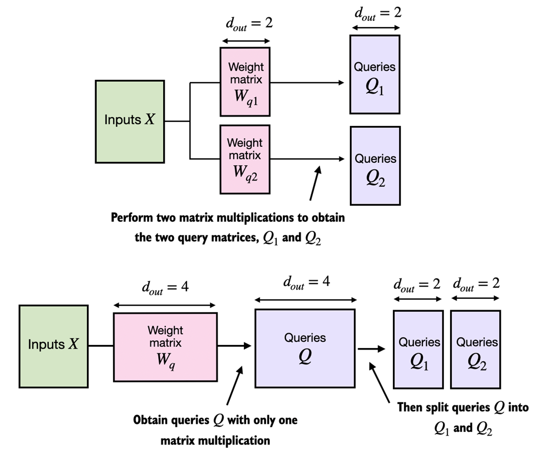
In the MultiheadAttentionWrapper class with two attention heads, we initialized two weight matrices Wq1 and Wq2 and computed two query matrices Q1 and Q2 as illustrated at the top of this figure. In the MultiheadAttention class, we initialize one larger weight matrix Wq , only perform one matrix multiplication with the inputs to obtain a query matrix Q, and then split the query matrix into Q1 and Q2 as shown at the bottom of this figure. We do the same for the keys and values, which are not shown to reduce visual clutter.

• Attention mechanisms transform input elements into enhanced context vector representations that incorporate information about all inputs.
• A self-attention mechanism computes the context vector representation as a weighted sum over the inputs.
• In a simplified attention mechanism, the attention weights are computed via dot products.
• A dot product is just a concise way of multiplying two vectors element-wise and then summing the products.
• Matrix multiplications, while not strictly required, help us to implement computations more efficiently and compactly by replacing nested for-loops.
• In self-attention mechanisms that are used in LLMs, also called scaled-dot product attention, we include trainable weight matrices to compute intermediate transformations of the inputs: queries, values, and keys.
• When working with LLMs that read and generate text from left to right, we add a causal attention mask to prevent the LLM from accessing future tokens.
• Next to causal attention masks to zero out attention weights, we can also add a dropout mask to reduce overfitting in LLMs.
• The attention modules in transformer-based LLMs involve multiple instances of causal attention, which is called multi-head attention.
• We can create a multi-head attention module by stacking multiple instances of causal attention modules.
• A more efficient way of creating multi-head attention modules involves batched matrix multiplications.

FAQ