7 Knapsack Algorithm

The knapsack problem is presented as a classic optimization challenge: given a fixed capacity and a set of indivisible items, the goal is to choose the combination with the greatest total value without exceeding the limit. The chapter contrasts this with earlier matching and string-search problems, then shows why a brute-force search is impractical because the number of possible item combinations grows exponentially. Since each choice is binary, take or leave, the problem naturally fits the 0/1 model, where partial items are not allowed and overlapping subproblems appear repeatedly.

To solve this efficiently, the chapter uses dynamic programming with a two-dimensional table whose rows represent how many items are considered and whose columns represent capacity from zero up to the maximum. The table is initialized with zeroes for the base cases, and each cell is filled by comparing two possibilities: skip the current item and inherit the value from above, or take the item and add its value to the best result from the remaining capacity. Working through a small example step by step shows how the table reuses previous results, avoids redundant computation, and gradually builds toward the optimal total rather than guessing locally best choices.

The chapter then connects the method to real-world resource allocation problems such as server scheduling and cargo loading, where hard limits and all-or-nothing decisions are common. It emphasizes that greedy methods can fail for 0/1 knapsack because the best-looking item may block a better overall combination, while fractional knapsack is different because greedily taking the highest value-to-weight ratio works there. Finally, it notes that the standard dynamic programming solution has time and space complexity of O(nW), which is practical for moderate capacities but becomes expensive when the capacity value itself is very large, motivating space optimization with one-dimensional arrays or alternative approximate methods when necessary.

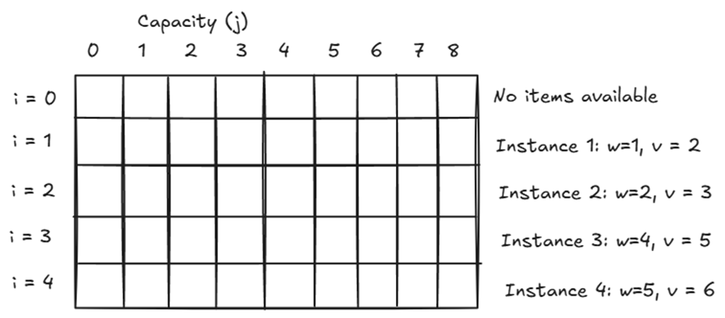
Initial 2D empty matrix with dimensions as (n + 1) x (W + 1), resulting in a 5 x 9 grid containing 4 items/instances and a maximum capacity of 8. The rows indicate the cloud instances available, while the columns show the incremental resource capacity to be considered to solve the problem.

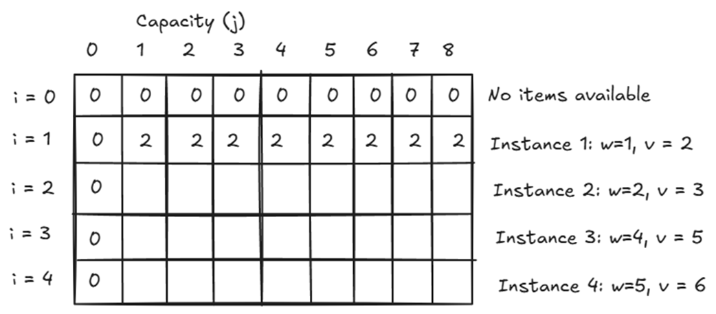
The matrix after executing boundary initialization and the first row iteration loop. Row i = 0 and column j = 0 are completely populated with zeroes, establishing the baseline conditions where zero value can be generated due to a lack of available items or a lack of capacity. Row i = 1 demonstrates horizontal state propagation for Instance 1 (w1 = 1, v1 = 2). Because this is a 0/1 Knapsack problem where multiple copies of the same item cannot be purchased, the optimal achievable throughput value levels out and remains exactly 2 across all subsequent capacity columns once the initial item cost is satisfied.

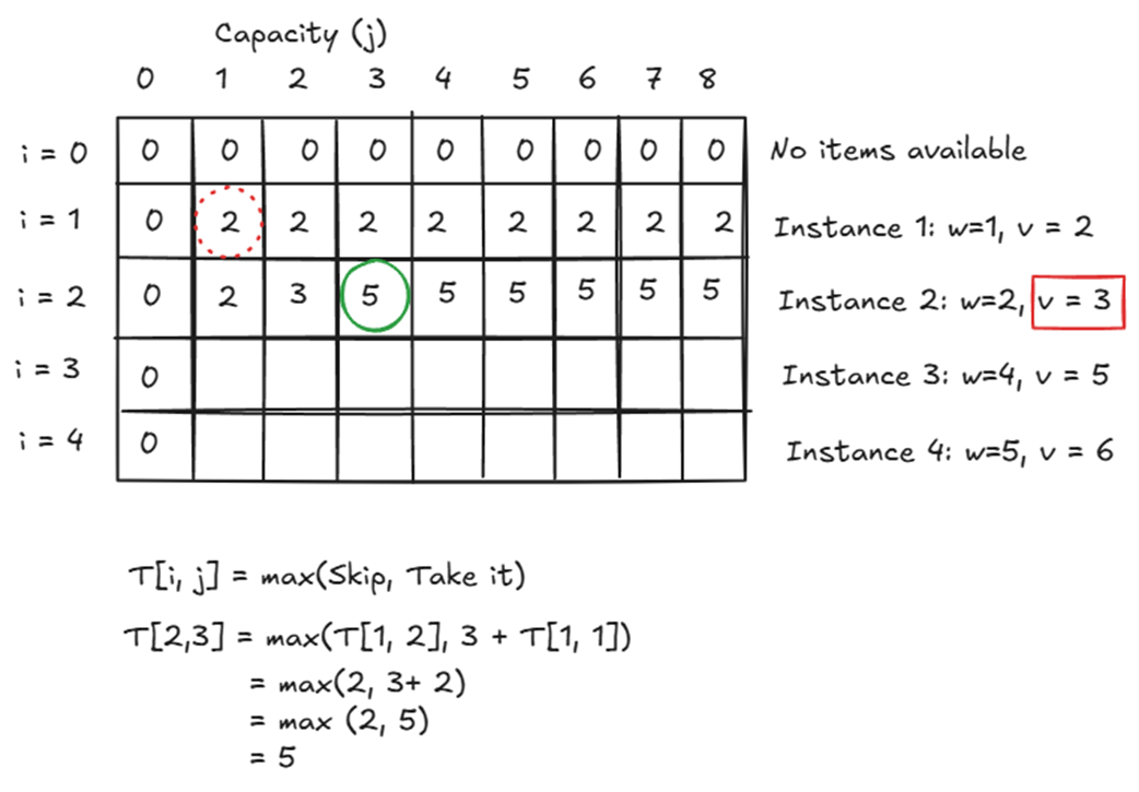
Visualization of the math used to evaluate cell T[2, 3] (circled in green) on the second row (w2 = 2, v2 = 3). The algorithm resolves a binary choice by executing a maximum value comparison between two paths. The exclusion path inherits the value directly above (T[1, 3] = 2). The active inclusion path accepts the new instance's throughput value (v2 = 3, highlighted in the red solid box) and subtracts its weight from the current capacity (3 - 2 = 1), forcing a pointer lookup to the previous row at column 1 (T[1, 1] = 2, highlighted by the red dotted circle). The combined value of 5 outperforms the exclusion path, updating the cell state.

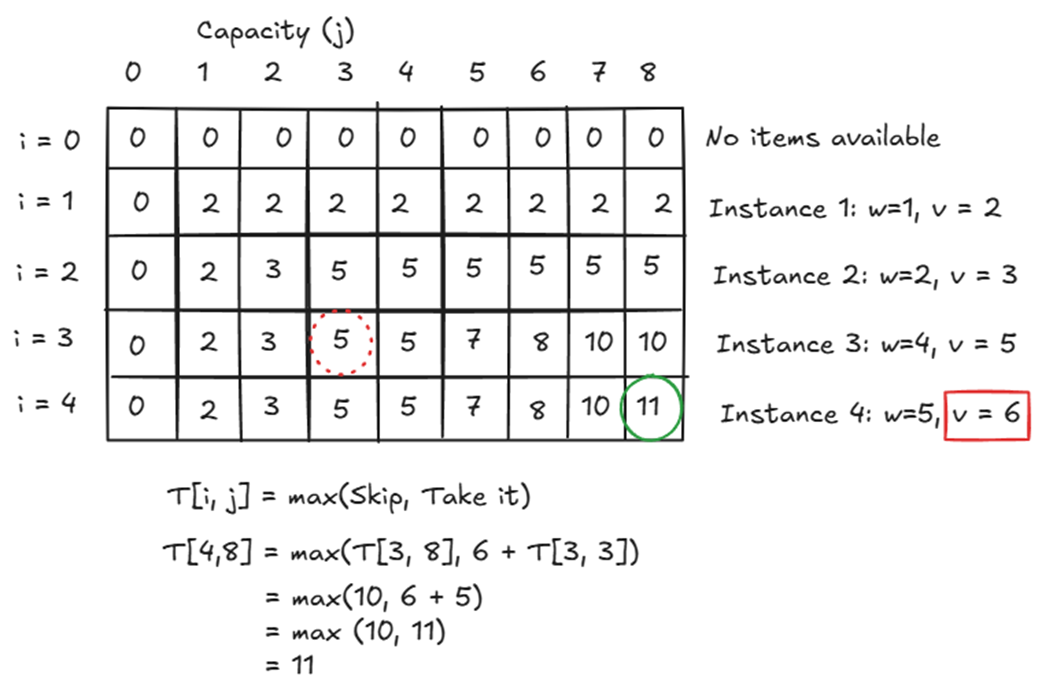
The final completed dynamic programming matrix highlighting the state evaluation for the absolute terminal cell, T[4, 8] (circled in green). At full resource capacity (j = 8) and looking at the final instance (w4 = 5, v4 = 6), the system checks its last binary fork. Skipping the instance yields a value of 10 from the row above. Taking the instance yields its standalone value of 6 plus the historical remaining capacity value found by looking backward 5 columns to the left at cell T[3, 3] (indicated by the red dotted circle containing a value of 5). The resulting sum (6 + 5 = 11) sets the global optimum for the entire problem.

• The 0/1 Knapsack problem is a foundational algorithmic framework designed to maximize total utility or performance value within a strict, unyielding capacity limit.
• It maps perfectly to scenarios where options are entirely binary and mutually exclusive, every resource choice requires an absolute 0/1 decision, meaning you must either fully commit to including an item (1) or exclude it entirely (0).
• Standard naive recursive approaches to subproblem optimization exhibit an exponential worst-case runtime complexity of O(2n) because the system lacks structural memory.
• Dynamic Programming completely eliminates this redundant overhead by permanently caching intermediate localized selections.
• To track state transitions systematically, the algorithm establishes a two-dimensional grid structured with a size of (n + 1) x (W + 1), where n represents the total available item count and W scales across every incremental unit of sub-capacity
• Every cell within the dynamic programming table, denoted as T[i, j], represents a concrete, localized global optimum for a restricted version of the overall challenge
• The algorithm populates the table coordinates by executing a strict binary evaluation at each cell using the formula T[i, j] = max(T[i-1, j], vi + T[i-1, j - wi]).
• The system weighs two distinct historical pathways: it checks the direct cost of skipping the item by reading the cell immediately above it, or it calculates the value of taking the item by combining its standalone profit with the historical optimal value of the leftover resource budget, found by stepping backward to the left by exactly the item's weight in the previous row.
• The performance metrics for a classic 2D matrix deployment scale with a time complexity of O(nxW) and a space complexity of O(nxW).
• The necessity of the dynamic programming matrix hinges entirely on the structural constraint of item indivisibility. If a problem context involves continuous, divisible commodities such as liquid fuels, raw grains, or loose manufacturing materials the 0/1 matrix framework is entirely bypassed in favor of the Fractional Knapsack model.
• While a comprehensive two-dimensional matrix is an excellent tool for analytical tracing and academic verification, it introduces an unnecessary space liability in memory-constrained production environments.

1. Code implementation: https://github.com/aniketwattamwar/Algorithms-Every-Programmer-Should-Know

FAQ