1 The Language of Algorithms

Algorithms are presented as the hidden machinery behind modern software and AI, shaping everything from apps and websites to large-scale systems that users depend on without noticing. The chapter frames them not as abstract classroom puzzles, but as practical ways of thinking that help programmers understand how software works under the hood. It emphasizes that learning algorithms is about building intuition, recognizing patterns, and being able to explain solutions clearly in plain language.

The chapter explains that an algorithm is a generalized step-by-step method for solving a well-defined problem, and that different algorithms can produce the same result with very different tradeoffs. It stresses why algorithms matter: they affect performance, reliability, scalability, and ultimately user experience. The discussion also highlights an important mindset for developers—real systems often value correctness, maintainability, and good judgment over unnecessary cleverness or premature optimization.

The text then introduces the foundations of algorithm analysis and essential data structures. Time and space complexity are used to judge efficiency, with worst-case behavior, Big O notation, and common growth rates such as constant, linear, quadratic, and logarithmic time explained through familiar examples like searching and sorting. It also shows how the choice of data structure changes what an algorithm can do efficiently, covering hash maps, linked lists, stacks, queues, trees, and graphs, along with traversal ideas like DFS and BFS, and illustrating how these structures support real-world tasks such as counting, navigation, scheduling, and network exploration.

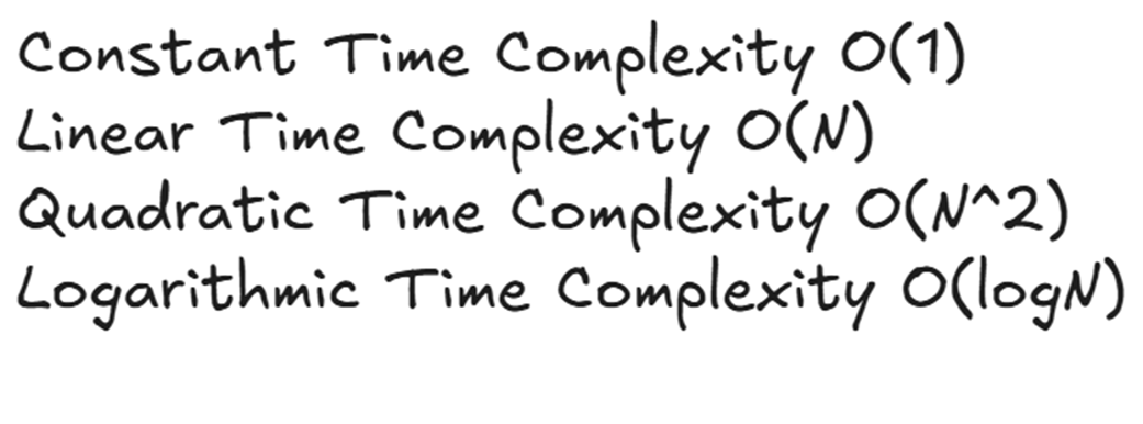
List of categories of time complexity used in algorithm analysis, including constant time O(1), linear time O(N), quadratic time O(N^2), and logarithmic time O(logN). N represents the increasing input size, highlighting the performance differences in time complexities.

A graph showing the time complexities with varying inputs. O(1) is the constant time, while O(n!) shows the worst time. O(log n) is logarithmic, and O(n) is linear time. Quadratic and cubic are in between and work well for smaller values of n.

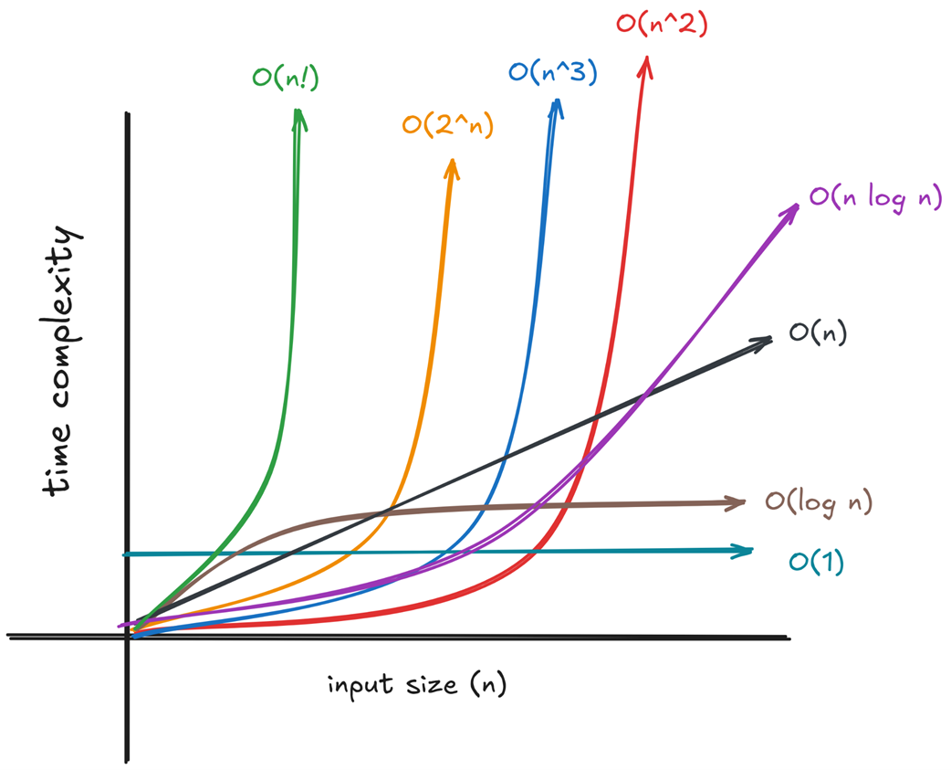
Illustration of a hash map where each key is associated with a list of values. Key1 maps to a list of numbers. Key2 maps to an empty list. The lists can be accessed via keys, which are unique in the hash map.

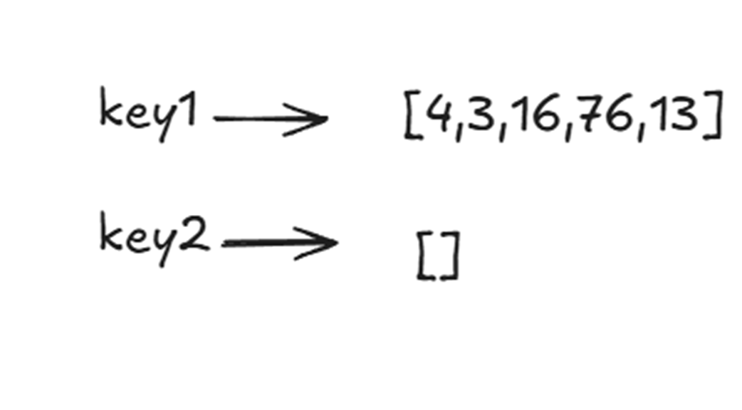
Illustration of a linked list with four nodes. Each node has data and a pointer pointing to the next node. The start of the linked list is marked as head. The end of the linked list is identified if the next pointer is null.

Illustration of a doubly linked list with 3 nodes. Each node has a previous pointer, data, and a next pointer. Doubly linked lists help in navigating both ways using the previous and next pointers.

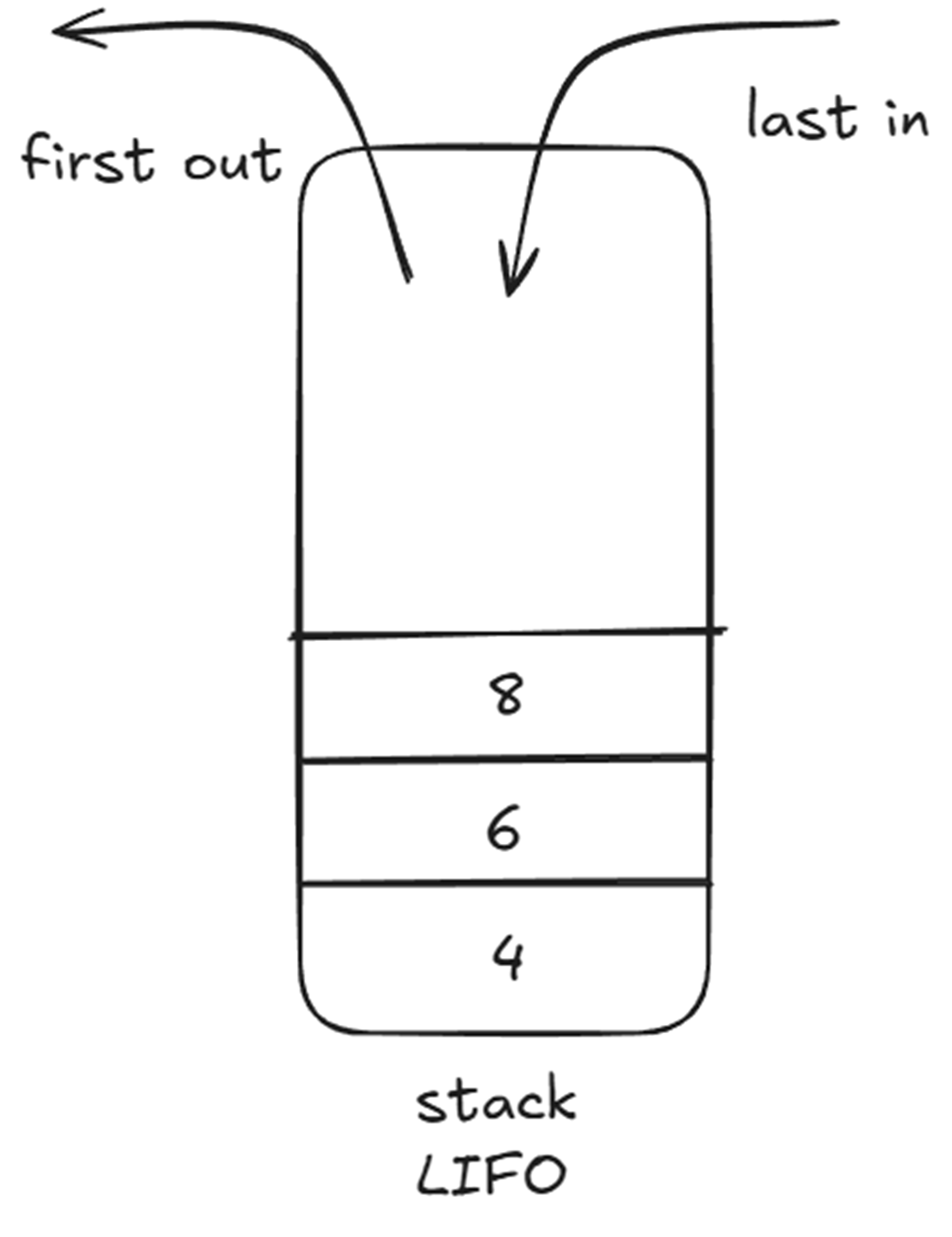
The stack data structure is Last In First Out(LIFO). Illustration of a stack with three numbers. The number 8 was inserted last and it will be popped first. The number 4 was inserted first, it will be popped only when all the numbers above the stack are popped first.

The queue data structure is First In First Out(FIFO). The number 8 illustrated in the image was inserted first, and it will be popped out first.

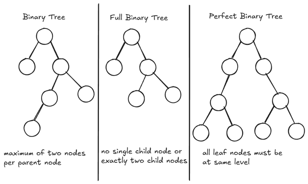
A comparison of common binary tree structural variations. Left: A standard binary tree where nodes have a maximum of two children. Middle: A full binary tree enforcing that nodes possess either exactly zero or exactly two child nodes. Right: A highly uniform perfect binary tree where all interior nodes contain two children and every leaf node aligns at the exact same depth level.

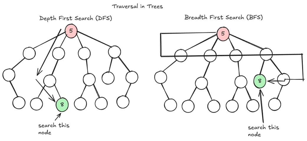
The two fundamental strategies for searching non-linear data structures. Left: Depth-First Search (DFS) goes deep down a single path to a leaf node. Right: Breadt-First Search (BFS) expands outward, exploring all the neighboring nodes layer by layer before descending to the next level.

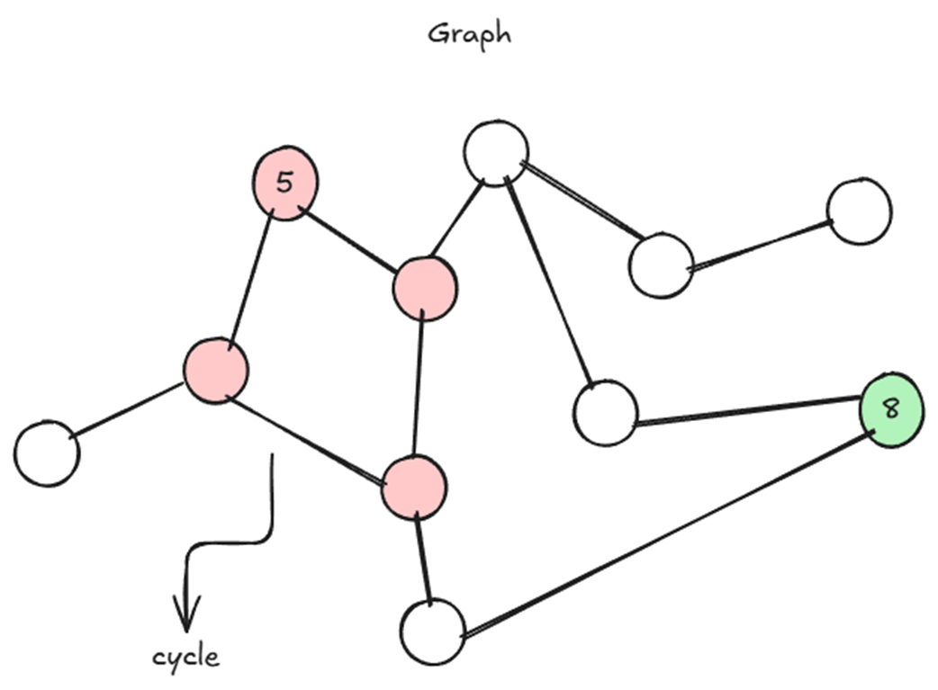
The transition from a tree to a relational graph. The structural tree rules are broken to form a cycle or a closed loop. One node can be connected to multiple nodes.

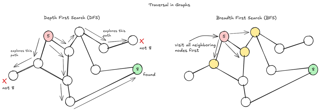
Traversal paths shown through a network with a cycle. Left: Depth-First Search (DFS) traces deep pathways until it detects dead-ends and mismatches. Right: A Breadth-First Search (BFS) expands to all neigboring or adjacent nodes. Both traversals use a visited set to track already visited nodes to avoid infinite loops.

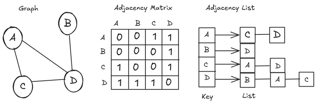
The two primary data structures for graph traversals. Left: Simple graph representation with four nodes connected to each other. Middle: An adjacency matrix maps connections from one node to another, denoting them by the value 1 in the matrix and otherwise 0. Right: An adjacency list showing a key-value dictionary connecting to neighboring nodes only.

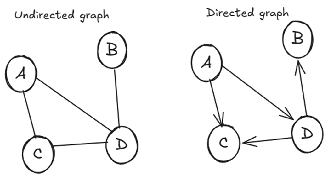
Two structural variations of a graph. Left: An Undirected Graph maps mutual, bidirectional connections. Right: A Directed Graph restricts travel paths to be unidirectional, forcing algorithms to explore a path based on direction.

• Algorithms govern the world of computer science. They are the fundamental blocks of software development. The design of algorithms should provide a general solution to inputs.
• An algorithm is a step-by-step procedure to be followed to arrive at a solution of a specified given problem
• Algorithms are needed, as they solve complex problems in multiple industries like healthcare, manufacturing, e-commerce, and more. Real-world systems rely on well-developed and scaled algorithms.
• Efficiency matters because slow and memory-heavy solutions break. Worst-case analysis is used generally to understand algorithm behavior, as it is the upper bound of performance. Best, worst, and Average time complexities are used for analysis of algorithms
• Common time complexities are constant time, linear time, quadratic time, and logarithmic time. Input N to these analyses shows the change in behavior of the output of the complexities.
• Data structures used influence algorithm performance. Arrays, linked lists, doubly linked lists, hash maps, stacks, and queues are a few data structures.
• Hashmaps store key-value pairs. They perform operations like insert, delete, and retrieval in O(1) time. They do not maintain order.
• Linked lists and doubly linked lists store data with pointers pointing forward and backward. This helps in traversal, and insertions and deletions are faster. Stacks and queues perform add and pop operations.
• Trees are hierarchical data structures for top-down, non-linear dependencies. Trees have a root node with multiple nodes attached to it called children, and those child nodes again have multiple nodes branching out. A node with no children is called a leaf node. The path from the root node to the leaf node is called the depth of a tree.
• Tree algorithms leverage constraints on the structure for predictability. Based on these constraints, types of trees are binary trees, full binary trees, and perfect binary trees.
• Binary Trees limit parents to a maximum of two children. A full binary tree permits nodes to have exactly two or zero children. Perfect binary trees are entirely symmetrical with all leaf nodes at the same depth level.
• Two traversal techniques exist: Depth First Search (DFS) and Breadth First Search (BFS). Breadth-First Search (BFS) utilizes a FIFO queue to sweep horizontally, level-by-level, expanding outward, bounding space complexity to the tree's width (O(W)). Depth-First Search (DFS) utilizes a LIFO stack to aggressively plunge vertically down a single branch before backtracking, bounding space complexity to the tree's depth (O(D)). Both track at O(V) time.
• Graphs are a network of nodes connected to each other but do not have constraints like trees. Any node can link to any other and contains loops and cycles. Algorithms must integrate an explicit visited set to track traversed nodes in a graph to avoid infinite loops. Time complexity of a graph is O(V + E), where V is the total number of vertices and E is the total number of edges or connections.
• Graphs use an adjacency matrix, a 2D array where the rows and columns are the vertices of the graph, a connection between two nodes is denoted by 1 or else 0, and an adjacency list, a memory-efficient key-value dictionary, where the keys are the vertices and the values represent the keys it's connected to.
• Connections in graphs are bidirectional or directional, called undirected graphs or directed graphs, respectively.

FAQ